Motivations
Basic GPT-2
Recently, I rewrote GPT2 as an exercice to help me prepare for big AI companies interviews. After reading the paper and reused the Shakespeare dataset given by Karpathy in its nanoGPT project, I started to write the code for the whole model :
- LayerNorm
- Attention layer
- Training loop
- Feed forward network (FFN)
- Positional embedding
Model improvements
I then focused on improving the model by implementing a few features such as :
- Multi Head Attention
- Multi Query Attention
The result was pretty satisfying. Of course, the dataset I am working with is character level tokenized, which is different from the tokenization that is used for regular LLMs. But the point was to build a fully functional POC, and I am pretty happy with what I have.
Inference
Now that I have a trained model, I want to make it produce tokens. I then worked on a key feature of language models : the KV-cache. The KV-cache is a way of only computing what is necessary at each generation step by storing what has already been computed somewhere, and reuse it to speed up the inference process. This is done as well, and indeed, it decreases a lot the inference time.
Hardware
What could be a next interesting step ? Training a large scale model requires a solid infrastructure, and lots of GPUs. A GPU is basically a piece of hardware that can run many operations simultaneously (this will be explained later in the article).
GPUs are expensive, and any company buying them wants to make sure they are used as efficiently as possible. And it turns out this is not as easy as it might seem.
For a GPU to be used efficiently, the programmer needs to understand a few concepts about how GPU are built, how they handle memory and I/O operations, and how to optimize the code for them.
This is what we are going to talk about today.
The following parts are mostly interesting things that I learnt while coding the model, fine tuning other models, trying different sets of hyperparameters…
Generalities
First, let’s give some general information about the inner workings of GPUs, data types, what needs to be stored in memory during training.
Data types
Model weights, optimizer states, gradients… are “just” numbers stored somewhere on the computer’s memory. But in a computer, it is possible to store number in different formats, and it matters for 2 reasons :
- Some formats take more space than others
- Some formats have a better precision that others (meaning they can represent numbers, and especially float more precisely)
Here are a the formats that can be used :
| Format | Total bits | Sign | Exponent | Mantissa |
|---|---|---|---|---|
| float32 | 32 | 1 | 8 | 23 |
| float16 | 16 | 1 | 5 | 10 |
| bfloat16 | 16 | 1 | 8 | 7 |
| float8 (e4m3) | 8 | 1 | 4 | 3 |
| float8 (e5m2) | 8 | 1 | 5 | 2 |
Let me explain what those figures mean. The first column is the number of bits a number stored in that format is going to take. We can see it in the name of the data type itself. float32 takes 32 bits in memory. The 3 other columns represent the number of bits taken by each part of the floating-point representation.
From Wikipedia :
In memory, numbers are stored using the scientific notation. In the scientific notation, the given number is scaled by a power of 10 so that it lies within a specific range (usually 1 and 10) with the radix point appearing immediately after the first digit. As a power of 10, the scaling factor is then indicated separately at the end of the number. For example, the orbital period of Jupiter’s moon Io is 152,853,5047 seconds, a value that would be represented in standard-form scientific notation as $1.528535047 \times 10^5$.
Floating point representation is similar, and a floating-point number consists of :
- A sign bit : whether the number of positive or negative
- An exponent : the scale at which the number is multiplied (5 in the example given by Wikipedia). 8 bits can store values from 0 to 255, but we need values that are greater than 1 as well as values that are between 0 and 1, so the exponent might be positive or negative, this will be clearer in the formula below
- A mantissa (or significand precision) : the radix of the number
Once we have the values of those 3 components, we compute the number as follow :
$$ \text{value} = (-1)^{\text{sign}} \times 2^{E - 127} \times (1 + \sum^{23}_{i = 1} b_{23 - i} 2^{-i}) $$
Which can be graphically represented by this schema from Wikipedia as well :
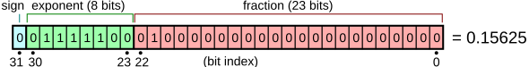
This one is for the float32 format, but other formats work the same way, with different precision for each part of the number.
Memory cost
Now that we have a better idea of how the numbers are actually stored in the memory, we need to understand what needs to be stored during training.
There are essentially 4 sets of numbers that are necessary :
- The model parameters : obviously, the weights of the models need to be available so that we can use them to compute outputs from inputs
- The gradients : the gradients are the updates we have to make to the model weights to converge towards a better solution. Note that the gradients have the same shapes as the parameters
- The activations : the activations are the intermediary outputs of the inner layers of the model, they are necessary to compute gradients so they have to be stored in memory as well, but since they are simply the outputs of inner layers, it is possible to recompute them if we don’t want to store them
- The optimizer states : information about the weights such as standard deviation, momentum, this depends heavily on what optimizer you use, SGD, Adam, AdamW…
It is important to note that all those sets of numbers do not have to be stored using the same float-point format. Some can be stored using float32 while others are stored using bfloat16 for instance.
To have an idea of the relative requirements for those different sets, let’s take a regular transformer-based model and give the memory needed based on a few parameters such as the number of layers, the hidden dimension, the context size…
- Input tokens : Each batch → $n \times b$
- Activations (hidden states) : For a single layer, the hidden state tensor → $n \times b \times h$, $h$ being the hidden dimension
- Model weights and gradients : Each layer is about $h^2$ elements, and gradients have the same size
- Optimizer states : Depends on the algorithm. Adam will keep :
- Variance and momentum in FP32 precision → $2 \times 2h^2$
- Master weights → $2 \times h^2$
- Total model parameters :
- Attention parameters :
- QKV projections : $3 h ^2$
- Output projections : $h^2$
- MLP parameters :
- Gate up → $2 \times h \times 4h$ (2 matrices of size h * 4h)
- Gate down → $4h \times h$ (1 matrix of size 4h * h)
- Total per block → $16h^2$ with GLU MLP, $12h^2$ without
- Full model → $16h^2 \times \text{num layers}$ (with GLU)
- Additional parameters :
- Input embedding → $\text{vocab size} \times h$
- LM head → $\text{vocab size} \times h$
- Positional embedding → $\text{max seq length} \times h$
- Attention parameters :
So for a simple transformer LLM, the number of parameters is given by the following formula :
$$ N = h \times v + n \times (12h^2 + 13h) + 2 \times h $$
Which can be verified using the transformers library :
from transformers import GPT2Model

def count_params(model):
    params: int = sum(p.numel() for p in model.parameters() if p.requires_grad)
    return f"{params / 1e6:.2f}M"

model = GPT2Model.from_pretrained('gpt2')

print(model)
print("Total # of params:", count_params(model))
Which prints :
GPT2Model(
  (wte): Embedding(50257, 768)
  (wpe): Embedding(1024, 768)
  (drop): Dropout(p=0.1, inplace=False)
  (h): ModuleList(
    (0-11): 12 x GPT2Block(
      (ln_1): LayerNorm((768,), eps=1e-05, elementwise_affine=True)
      (attn): GPT2Attention(
        (c_attn): Conv1D()
        (c_proj): Conv1D()
        (attn_dropout): Dropout(p=0.1, inplace=False)
        (resid_dropout): Dropout(p=0.1, inplace=False)
      )
      (ln_2): LayerNorm((768,), eps=1e-05, elementwise_affine=True)
      (mlp): GPT2MLP(
        (c_fc): Conv1D()
        (c_proj): Conv1D()
        (act): NewGELUActivation()
        (dropout): Dropout(p=0.1, inplace=False)
      )
    )
  )
  (ln_f): LayerNorm((768,), eps=1e-05, elementwise_affine=True)
)
Total # of params: 124.44M
The requirements for the optimizer states depend heavily of what optimizer you are using for training.
For example the Adam optimizer requires information such as momentum and variance to be stored for each parameter, adding another 8 bytes per parameter.
Having even a rough idea of the relative costs of the different sets that we have to store in memory in interesting in many ways, and can sometimes be surprising.
For example, this chart is taken from the Ultra-scale playbook on the Huggingface website :
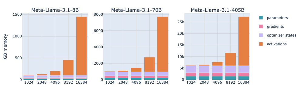
We can notice that the parameters of the model itself account for the most part as long as the context size is small, but they then become almost negligible from around 8-16k tokens.
This is mostly because the Attention memory increases quadratically with the sequence length, which at some point is going to be too much for our GPU to handle. Let’s keep that in mind.
Compute cost
As we understood from the chart above, the activations are going to be a serious issues if we plan on training a model that has a significant context size.
This allows me to point you, the reader, to an article I wrote a few weeks ago about gradient checkpointing, also called activation recomputation : https://bornlex.github.io/posts/ai-finetuning-learnings/.
Tokens
Compute number of tokens necessary to train a model.
GPU
Now that the requirements in terms of memory and tokens are clear in our head, we need to talk about the thing that made deep learning actually work : GPU.
Before AlexNet, a convolutional image classification model written by Alex Krizhevsky, Ilya Sutskever under the supervision of Geoffrey Hinton, deep learning models were trained using CPU. In 2012, for the ImageNet image classification context, they presented their network and won the context by a very large margin. The secret ? The model used a bigger depth, and thus required lots of computation to be trained. They used GPU, and the graphical computation library CUDA, to use the Nvidia graphical processor.
AlexNet is not the first GPU-trained model, a few models have been trained before using GPU.
In the following parts, I will be talking about the inner workings of current GPU, and how we can use their power to parallelize the computation and speed up training.
Compute
First, let’s discuss how GPUs operate on numbers.
A GPU is basically an array of compute units called streaming multiprocessors (SM). Each SM contains a set of streaming processors, often called cores.
A single core is capable of handling multiple threads simultaneously.
As an example, the NVIDIA H100 has 132 SMs with 128 cores each, so a total of 16,896 cores.
Memory
The memory of a GPU is hierarchical as well. Some parts of the memory is shared across SMs while others are not.
The smallest memory unit inside a GPU is called a register. Registers are private to the threads during execution.
Each SM contains a Shared Memory and a L1 Cache. They are shared between the threads that are running inside a single SM.
Finally, the GPU contains one L2 Cache and a Global Memory, both shared by all SMs. The global memory is the largest memory on the GPU, but also the slowest.

This is from the Huggingface Ultra Scale playbook.
Optimization
Obviously, when training our model, we want to make the most out of the GPUs we have. This means making sure as many workloads as possible are running in parallel on the available cores.
This means taking advantage of the knowledge we have on the way compute and memory work on the GPU.
A piece of code that runs on a core is called a kernel. For a kernel to run on a core, it needs to be compiled to Parallel Thread Execution (PTX) which is the assembly language used by NVIDIA GPUs. But kernels are mostly written in two higher programming languages :
- CUDA
- Triton
before being compiled to PTX.
For a kernel to run, it needs preparation from what is called the host code. The host code is executed on the CPU/host machine (in our case this is the Pytorch code for instance). The host code is responsible for :
- Preparing data allocations
- Loading data and code before execution
Running a kernel usually works as follow :
- Threads are grouped in warps (a group of 32 threads), warps are synchronised to execute instructions simultaneously but on different part of the data (for example different parts of a matrix)
- Warps are grouped in larger blocks of flexible size, and each block is assigned to a single SM
- Because a SM can have more threads than a block can contain, it can run multiple blocks in parallel
- That does not mean that all the blocks may get assigned immediately, depending on the resources available at any given moment, some blocks can be waitlisted for later execution
Memory Access
Finally, before digging into writing kernels with a famous example, let’s talk how memory is accessed.
Each time a DRAM location (global memory) is accessed, sequence of consecutive locations is returned. So instead of reading one location, we actually read a few locations at a time.
The idea behind this mechanism is to optimize memory access by ensuring threads in a warp access consecutive memory locations.
For example, if thread 0 reads location M, then thread 1 will get location M + 1, thread 2 → M + 2…
Writing kernels
After all those theoretical information, it is time to dig in what brings us here, make the GPU go brrr.
There are multiple ways of writing code that will be executed by the GPU (from the easiest to the hardest) :
- Use plain Pytorch
- Use @torch.compile as a decorator, on top of a function
- Use Triton : a Python library developed by OpenAI to wrap CUDA code directly inside Python
- Use CUDA : the NVIDIA library to execute code on the GPU
As an example, we will consider the softmax function, computed with only pytorch first, and then with a Triton implementation to show how this can improve execution performances.
Pytorch version
Let’s start by giving a Pytorch version of the softmax function :
import torch

def naive_softmax(x):
    x_max = x.max(dim=1)[0]
    z = x - x_max[:, None]
    numerator = torch.exp(z)
    denominator = numerator.sum(dim=1)
    ret = numerator / denominator[:, None]

    return ret
And some explanations about the shapes of the object loaded in memory. Considering that $x \in \mathbb{R}^{m \times n}$ (m rows and n columns) :
- Computing the max along the last dimension (the maximum value for all the rows) requires reading the whole matrix and writing back to memory the array of maximum values
- Read : $m \times n$
- Write : $m$
- Subtracting the max from the matrix and storing the result in a different matrix
- Read : $m \times n + m$
- Write : $m \times n$
- Computing the exponential of all elements of the matrix
- Read : $m \times n$
- Write : $m \times n$
- Computing the sum along the last dimension (the sum of the elements of each row)
- Read : $m \times n$
- Write : $m$
- Dividing the numerator (a matrix) by the denominator (a vector)
- Read : $m \times n + m$
- Write : $m \times n$
So the total of memory operations is :
- Read : $5mn + 2m$
- Write : $3mn + 2m$
Obviously, when we read a matrix from DRAM, compute the exponential function on it, store it, read it again to perform another operation, and so on, we are wasting time doing things on numbers that could have been kept in memory and wrote to DRAM at the very end.
Triton version
Let’s now give the Triton equivalent of the Pytorch code above, and explain a few things about the implementation, which seems very different from the plain softmax we computed earlier.
@triton.jit
def softmax_kernel(
		output_ptr,
		input_ptr,
		input_row_stride,
		output_row_stride,
		n_rows,
		n_cols,
		BLOCK_SIZE: tl.constexpr,
		num_stages: tl.constexpr
):
    row_start = tl.program_id(0)
    row_step = tl.num_programs(0)

    for row_idx in tl.range(row_start, n_rows, row_step, num_stages=num_stages):
        row_start_ptr = input_ptr + row_idx * input_row_stride

        col_offsets = tl.arange(0, BLOCK_SIZE)
        input_ptrs = row_start_ptr + col_offsets
        mask = col_offsets < n_cols
        row = tl.load(input_ptrs, mask=mask, other=-float('inf'))

        row_minus_max = row - tl.max(row, axis=0)
        numerator = tl.exp(row_minus_max)
        denominator = tl.sum(numerator, axis=0)
        softmax_output = numerator / denominator

        output_row_start_ptr = output_ptr + row_idx * output_row_stride
        output_ptrs = output_row_start_ptr + col_offsets

        tl.store(output_ptrs, softmax_output, mask=mask)
First let’s talk about the arguments :
- output_ptr : the pointer of the allocated space for the output matrix (the matrix that will contain the result)
- input_ptr : the pointer of the allocated space of the input matrix (the one we are computing the softmax on)
- input_row_stride : on memory, the elements of a matrix are contiguous, the first element of the second row is located right after the last element of the first row, so this argument is used to know the jump we need to make to get the next row, in our case this is simply the number of elements in one column
- output_row_stride : the same thing as before but for the output matrix
- n_rows : the number of rows of the matrix we compute softmax on
- n_cols : the number of columns of the matrix we compute softmax on
- BLOCK_SIZE : in this case, this is closest power of 2 higher than the number of columns
To illustrate what stride means precisely, let’s have a look at a 3 by 4 tensor :

This is a tensor of shape (3, 4), 3 lines and 4 columns, so 4 elements per line. Because the memory is a giant sequence of locations, this tensor is actually “flattened” when stored in memory. So when we are using Pytorch, the framework handles this for us, but now that we are interested in working directly with the memory, we have to understand that the tensor actually looks like this :

The first line elements are stored first, then directly after the last element of the first line comes the first element of the second line and so on.
So if we want to jump from the first line pointer to the second line pointer (from the location of the start of the first line to the location of the start to the second line), we have to know how many locations we are jumping. This is what stride is for.
In Pytorch, we can get this number with the :
x = torch.rand(3, 4)
x.stride(0)  # returns 4
This tells us how many locations we have to jump to go from an element to the next along the first dimension (0). In a 2d matrix, this is simply the shape of the second dimension, but it could be different when working with bigger tensors such as (3, 4, 3) for instance :
x = torch.rand(3, 4, 3)
x.stride(0)  # returns 12 = 4 x 3 because we have to jump 2 dimensions
Now let’s explain the first two lines of the program, they are very specific to writing kernels :
row_start = tl.program_id(0)
row_step = tl.num_programs(0)
To understand what we use these two lines, recall how the GPU works. The kernel is not going to run on the whole matrix and iterate over the rows like a regular program would. Instead, multiple instances of this kernel will run in parallel, each working on a different row of the input matrix. When we are in a specific instance, we need to know on what row we are going to be operating. The first line gives the first row the current kernel instance will operate, and the second line returns the step, which is basically the number of programs that will run in parallel.
So the first kernel instance will run on row 0, the second instance on row 1, and so no until we reach the total number of instances running, let’s say 64, and so the first kernel instance will have to work on row 64 after it finished working on row 0.
This logic explains why we have to iterate from row_start to n_rows, with a step of row_step.
The first line of the loop is used to get the pointer of the first element of the current row. Since we know the location of the matrix in memory (input_ptr), the size of 1 row and the index of the current row, we can easily get the location of the row in memory.
The four lines that comes after are used to load the entire row in memory :
col_offsets = tl.arange(0, BLOCK_SIZE)
input_ptrs = row_start_ptr + col_offsets
mask = col_offsets < n_cols
row = tl.load(input_ptrs, mask=mask, other=-float('inf'))
The col_offsets is used to create indices from 0 to BLOCK_SIZE and we then masks the indices that are higher than the maximum column index.
The four following lines are simply where we compute the softmax function itself, they are very straightforward and look like the pytorch version a lot :
row_minus_max = row - tl.max(row, axis=0)
numerator = tl.exp(row_minus_max)
denominator = tl.sum(numerator, axis=0)
softmax_output = numerator / denominator
The last 3 lines are similar to what we did when loading the row from the input matrix :
output_row_start_ptr = output_ptr + row_idx * output_row_stride
output_ptrs = output_row_start_ptr + col_offsets

tl.store(output_ptrs, softmax_output, mask=mask)
but this time with the output matrix.
Conclusion
To conclude, the Triton kernel is not too far from the Pytorch version for this simple softmax implementation. It is basically a row by row softmax implementation, with the read/write from/to memory on top of it.
For more complex algorithms, such as the very famous FlashAttention kernel, things might get a bit more complicated, but let’s keep this for a later article !
Resources
- https://www.harmdevries.com/post/context-length/
- https://huggingface.co/spaces/nanotron/ultrascale-playbook
- https://en.wikipedia.org/wiki/Floating-point_arithmetic
- https://michaelwornow.net/2024/01/18/counting-params-in-transformer
- https://arxiv.org/abs/2205.14135
- https://triton-lang.org/main/index.html
- https://blog.codingconfessions.com/p/gpu-computing
- https://siboehm.com/articles/22/CUDA-MMM