Introduction

Neural networks require large amounts of data to converge. Those data need to represent the task the neural network is trying to learn.

Data collection is a tedious process, especially when collecting data can be difficult or expensive. In science, physics for instance, many phenomenon are described using theories that we know are working very well.

Using those data as regularization can help neural networks generalize better with less data.

In some area, like fluid dynamics, using statistical models can speed up simulations and avoid using computationally expensive system of equations (Navier Stokes for instance).

When trying to predict the behavior of a physical system, we most of the time want to know the state of the system at a certain point in time $t$. We are looking an equation that looks like this:

$$ x(t) = f(t; \theta) $$

Here $x$ is the true phisical state of the system at time $t$ and $f$ is our neural network that will approximate it. It is parametrize by $\theta$, the weights.

Of course, we will use some data that we collected in order to fit our model. This will look like a typical training, with a loss:

Of course, we will use some data that we collected in order to fit our model. This will look like a typical training, with a loss:

$$ L(\hat{Y}, Y) = \frac{1}{N} \sum^N_i(\hat{y}_i, y_i)^2 $$

Where:

• $\hat{y}_i \in \hat{Y}$ is a prediction made by the model
• $y \in Y$ is the set of ground truth

Of course, this is equivalent to:

$$ L(\hat{Y}, Y) = \frac{1}{N} \sum^N_i(f(t_i; \theta), y_i)^2 $$

But, because we want our model to follow the dynamics of a real physical system, we can insert into the loss a regularization term that corresponds to a physical equation.

Let us give a concrete example of a regularization term that corresponds to a real physical equation.

Spring-mass System

Context

Let us imagine the following situation: we have a spring-mass system on a table and we want a model that will predict the position of the system at any point in time $t$.

We note the real trajectory of the system $t \mapsto x(t)$.

Because finding the exact solution might be difficult analytically (for the spring-mass system, the solution is actually not so difficult, so we could reach it analytically, but for some other systems it might not be that easy), we want a model that will predict the state of the system. To do this, we choose a neural network.

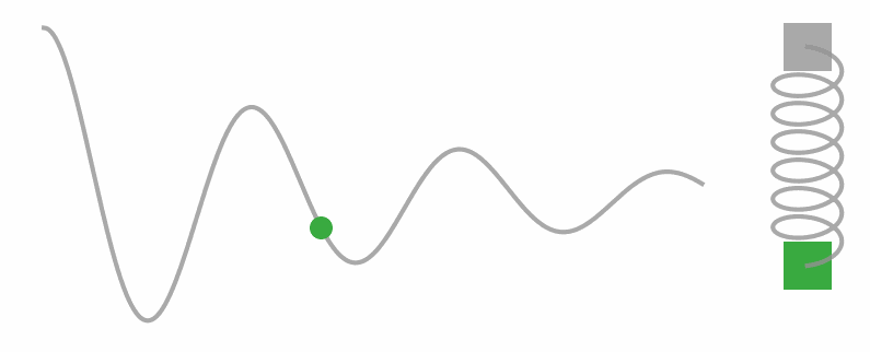
The grey line represents the position of the mass (the green square) over time. The green dot is the position at time $t$.

Here, the problem we have is that the data we collected are all located at the beginning of the phenomenon. The risk here is that we get a decent approximation until we reach the last point in time that we measured and after that, the network might behave strangely.

The orange dots are the measures we collected.

Let us notice that the mass is dampened, which might be not so easy to teach our neural network to replicate.

This is why we will have to introduce to our neural networks some physical lessons.

Differential equation

Let us do some good old physics here by applying the Newton law:

$$ \sum_i \overrightarrow{F}_i = m\overrightarrow{a}_G $$

The forces that take place here are:

• the weight $\overrightarrow{P}$
• the spring opposing force $\overrightarrow{F}$, that depends on how much the spring is elongated (Hooke’s law)
• friction $\overrightarrow{f}$, depends on the speed of the spring-mass system
• vertical reaction of the table on the spring-mass system $\overrightarrow{R}$

The spring-mass system not being very heavy, the vertical reaction of the table and the weight are cancelling each other.

Moreover, we are interested in the horizontal position of the spring-mass system, so we can project our equation on the horizontal axis and ignore those two forces.

Our differential equation then becomes:

$$ F + f = m a_G $$

Which then becomes:

$$ -kx(t) - \alpha \dot{x}(t) = m \ddot{x}(t) $$

Then:

$$ m \ddot{x}(t) + \alpha \dot{x}(t) + kx(t) = 0 $$

And finally:

$$ \ddot{x}(t) + \frac{\alpha}{m} \dot{x}(t) + \frac{k}{m}x(t) = 0 $$

This is a second order differential equation on the position of the spring-mass system $x(t)$.

Regularization

Now that we have the differential equation for our system, we can use it to train our model. The easy way to use it during training is the loss function.

We can see it as a regularization term. We need our model to predict correctly the measures and to respect the dynamics given by the differential equation.

Those two constraints are going to be enforced the same way: by computing the mean square error with the expected value.

Our loss function will look like this:

$$ L = \frac{1}{N} \sum^N_i (y_i - f(x_i) )^2 + \lambda \frac{1}{N} \sum^N_i [\ddot{f}(x_i) + \frac{\alpha}{m} \dot{f}(x_i) + \frac{k}{m} f(x_i)]^2 $$

In order to compute the first order and second order derivatives in the second term, you will have to use the torch.autograd.grad function of the pytorch library two times, one for the first order derivative, and a second time for the second order derivative.

The $\lambda$ parameter is a weighting parameter.

Practicum

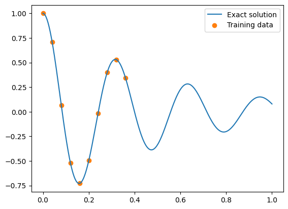
In order to train our neural network, we need to generate some synthetic data and sample some out of it:

def oscillator(d, w0, x):
    assert d < w0
    w = np.sqrt(w0 ** 2 - d ** 2)
    phi = np.arctan(-d / w)
    A = 1 / (2 * np.cos(phi))
    cos = torch.cos(phi + w * x)
    sin = torch.sin(phi + w * x)
    exp = torch.exp(-d * x)
    y  = exp * 2 * A * cos
    return y

d, w0 = 2, 20
mu, k = 2 * d, w0 ** 2. # the alpha/m and k/m constants in the reg term

# generate some synthetic data
x = torch.linspace(0, 1, 500).view(-1, 1)
y = oscillator(d, w0, x).view(-1, 1)

# sample some data to train on
x_data = x[0:200:20]
y_data = y[0:200:20]

# display the dataset and sample used for training
plt.figure()
plt.plot(x, y, label="Exact solution")
plt.scatter(x_data, y_data, color="tab:orange", label="Training data")
plt.legend()
plt.show()

Display functions

Here is a function to display the results of your model:

def plot_result(x, y, x_data, y_data, yh, xp=None):
    """
    x: the xs dataset
    y: the ys dataset
    x_data: the data used for prediction: t
    y_data: the ground truth x(t)
    yh: the prediction of the model: f(t)
    """
    plt.figure(figsize=(8, 4))
    plt.plot(x, y, color="grey", linewidth=2, alpha=0.8, label="Exact solution")
    plt.plot(x, yh, color="tab:blue", linewidth=4, alpha=0.8, label="Neural network prediction")
    plt.scatter(x_data, y_data, s=60, color="tab:orange", alpha=0.4, label='Training data')
    if xp is not None:
        plt.scatter(
            xp, -0 * torch.ones_like(xp), s=60, color="tab:green", alpha=0.4,
            label='Physics loss training locations'
        )
    l = plt.legend(loc=(1.01, 0.34), frameon=False, fontsize="large")
    plt.setp(l.get_texts(), color="k")
    plt.xlim(-0.05, 1.05)
    plt.ylim(-1.1, 1.1)
    plt.text(1.065, 0.7,"Training step: %i"%(i+1),fontsize="xx-large",color="k")
    plt.axis("off")

Model

We will use a simple PyTorch neural network:

class SimpleNN(nn.Module):
    def __init__(self):
        super().__init__()
        self._fc1 = nn.Linear(1, 32)
        self._fc2 = nn.Linear(32, 32)
        self._fc3 = nn.Linear(32, 1)
        self._activation = nn.Tanh()

    def forward(self, x: torch.Tensor):
        x = self._fc1(x)
        x = self._activation(x)
        x = self._fc2(x)
        x = self._activation(x)
        x = self._fc3(x)
        return x

Training

Most of the work (actually the regularization term) will be held inside the training function. You will need to use the autograd.grad function in order to compute the first order and the second order derivatives.

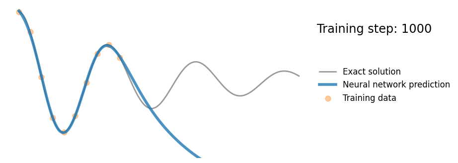
Regular neural network

In order to compare the results with and without this regularization term, we will start by training a neural network without with only the MSE loss.

At the end of training with parameters:

• $lr = 1.10^{-3}$
• $epochs = 10^3$

model = SimpleNN()
optimizer = torch.optim.Adam(model.parameters(), lr=1e-3)

for i in range(1000):
    optimizer.zero_grad()
    yh = model(x_data)
    loss = torch.mean((yh - y_data) ** 2) # MSE
    loss.backward()
    optimizer.step()

    if (i + 1) % 10 == 0:
        yh = model(x).detach()
        plot_result(x, y, x_data, y_data, yh)
        if (i + 1) % 500 == 0:
            plt.show()
        else:
            plt.close("all")

The prediction should look like this:

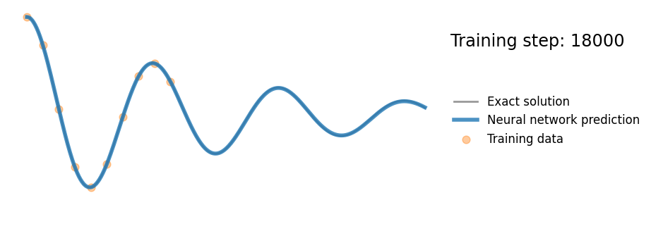
Physics informed neural network

Then we will train the same neural network but with the regularization term. Training will be done with parameters:

• $lr = 1.10^{-4}$
• $epochs = 2.10^4$

mu, k = 2 * d, w0 ** 2

physics_model = SimpleNN()
optimizer = torch.optim.Adam(physics_model.parameters(), lr=1e-4)

x_physics = torch.linspace(0, 1, 30).view(-1, 1).requires_grad_(True)

l = 1e-4

for i in range(20000):
    optimizer.zero_grad()

    yh = physics_model(x_data)

    loss = torch.mean((yh - y_data) ** 2)

    yh_phy = physics_model(x_physics)

    dx = torch.autograd.grad(yh_phy, x_physics, torch.ones_like(yh_phy), create_graph=True)[0]
    dx2 = torch.autograd.grad(dx, x_physics, torch.ones_like(yh_phy), create_graph=True)[0]
    regularization = dx2 + mu * dx + k * yh_phy
    regularization = torch.mean(regularization ** 2)

    loss_physics = loss + l * regularization # MSE + regularization

    loss_physics.backward()
    optimizer.step()

    if (i + 1) % 1000 == 0:
        yh = physics_model(x).detach()
        plot_result(x, y, x_data.detach(), y_data, yh)
        if (i + 1) % 6000 == 0:
            plt.show()
        else:
            plt.close("all")

As you can see in the loss function above, there is a $\lambda$ parameter, we can use $1.10^{-4}$ at first, it should give good results.

The regularization term will not be computed on the same values than the MSE loss term otherwise it might perturbate the computation graph.

So you will generate 30 points between 0 and 1 using torch.linspace. Do not forget to call the require gradient method on them, otherwise gradient won’t be computed during training.

At the end of training, you should see something like this:

Concept

Basically, what we are doing is choosing a class of function to approximate a phenomenon (the neural network), fitting it on data and adding a regularization term to ensure that our function respects conditions that are mandatory in real life.

This is why we can collect data only for the first seconds of the phenomenon, because we restricted our search for a solution to only solutions that respects Newton’s law, which makes the search much easier for our optimization algorithm.

Conclusion

This paradigm is the foundation for physics-based AI, such as the very impressive realization of Leap71 and their engine designed by AI.