Reinforcement Learning with Apple MLX Framework

Today, a very short article about Apple MLX framework.
I recently learned that Apple has its own machine learning framework, and as a heavy Mac user I thought I’d give it a try.
It is very easy to use and intuitive, the syntax is nice and looks like Numpy and PyTorch, which is convenient as a PyTorch user.
As an example, let me present a Deep Q Learning implementation that I wrote. It comes from a nice DeepMind paper.
Algorithm
Bellman equation
The algorithm itself is relatively simple, it learns the value of performing a specific action in a given environment state.
The function is learns to approximate is usually named $Q$, hence the name of the algorithm.
Let’s take the following notations:
- $a \in A$ an action belonging to the space of actions
- $\pi \in \Pi$ a strategy belonging to the space of strategies
- $s \in S$ a state belonging to the space of states (might be the position of a character in an environment, )
- $Q : S \times A \to \mathbb{R}$ the function that gives the value of playing an action $a$ in a state $s$, we sometimes note this function $Q_{\pi}$ because the value of choosing $a$ in state $s$ depends on what the agent is going to do after, which depends on the stategy it follows
Once we get these notations, we can introduce the core formula ruling DQN, the Bellman equation:
$$ Q_{\pi}(s, a) = r + \gamma \mathbb{E}[ \max_{a’} Q_{\pi}(s’, a’) | s, a] $$
Where we find the following additional terms:
- $r$ is the reward already accumulated at this point in the program
- $\gamma$ is a discounting factor, reducing the value of what is expected to be earned in the future, because it is not certain (in french we have a saying “un tiens vaut mieux que deux tu l’auras” meaning receiving one now is better that maybe receiving more tomorrow)
The formula is interpreted as: the value of playing action $a$ in the current state $s$ is the expectancy of what I already have now $r$ plus what I can get in the future if I play as good as I can.
Deep Q Learning
The DQN algorithm uses two models:
- an online model that will be trained regularly
- a target model that receives the online model parameters from time to time, to increase stability
The DeepMind paper gives the following pseudo code:
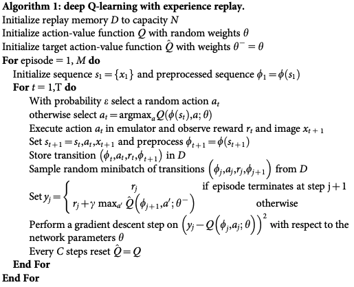
We see that the loss function is not directly the Bellman equation, but instead takes into account the difference between the prediction of the online network at time $t$ and what the target network predicts at time $t + 1$ after being discounted through the Bellman equation.
After each learning step, the online network copies its parameters into the target network and training continues.
Implementation
I am not going to give the full implementation (it is available from my Github, see the link in the reference section) but instead highlight some components and how they are written using MLX.
Environment
I used the CartPole-v1 environment available using the gymnasium Python library.
Model
The model is very simple and looks like a Pytorch model:
import mlx.core as mx
import mlx.nn as nn
import numpy as np

class Model(nn.Module):
    def __init__(self, environment):
        super().__init__()

        self.__environment = environment
        self.layers = self.build_network(
            int(np.prod(self.__environment.observation_space.shape)),
            int(self.__environment.action_space.n)
        )

    def build_network(self, state_size: int, action_size: int) -> list:
        return [
            nn.Linear(state_size, 64),
            nn.Tanh(),
            nn.Linear(64, action_size)
        ]

    def __call__(self, x):
        for layer in self.layers:
            x = layer(x)

        return x

    def act(self, observation):
        observation_tensor = mx.array(observation, dtype=mx.float32)
        q_values = self(observation_tensor)

        max_q_index = mx.argmax(q_values, axis=0)
        action = max_q_index.item()

        return action
This code could nearly be used as it is with PyTorch. MLX even used the same nn.Module notation as PyTorch.
Training
Initializing replay buffer
For our algorithm to train the first time, we need to initialize the experience buffer with some episodes that are played randomly, by sampling actions.
  def __init_replay_buffer(self):
      observation, _ = self.__env.reset()
      for _ in range(self.__args.min_replay_size):
          action = self.__env.action_space.sample()
          _, _, reward, new_observation, done = self.__step_env(
              action, observation
          )
          observation = new_observation

          if done:
              observation, _ = self.__env.reset()
This does not say much about MLX, but more about the nice gymnasium libraries and how to call environment.
Exploration vs Exploitation
The big dilemma in reinforcement learning is knowing when to optimize the outcome based on what you already know (exploitation) and when to try something else (exploration).
Technically, it means that sometimes, we are going to sample our next action randomly in order to populate the experience buffer which we learn with more variety.
  def __choose_action(self, epsilon, observation):
      if np.random.rand() < epsilon:
          return self.__explore()

      return self.__exploit(observation)
Epsilon is the argument that controls how much we explore. It decreases along the way so we focus more and more on the best actions over time.
Play
Once we know how to choose the next action, we can play a few episodes, add them to the replay buffer to train on later:
  def __behave(self, observation, step, episode_reward):
      epsilon = self.__compute_exploitation_exploration_tradeoff(step)

      action = self.__choose_action(epsilon, observation)

      _, _, reward, new_observation, done = self.__step_env(
          action, observation
      )
      observation = new_observation
      episode_reward += reward

      if done:
          observation, _ = self.__env.reset()
          self.__reward_buffer.append(episode_reward)
          episode_reward = 0.0

      return observation, episode_reward
Learn
Now that our replay buffer fills in, we can use it to learn the $Q$ function based on what we did.
This will introduce a mechanism in MLX that is different from PyTorch:
  def __learn(self, step: int):
      transitions = random.sample(self.__replay_buffer, self.__args.batch_size)
      observations, actions, rewards, new_observations, dones = self.__to_tensors(transitions)

      target_q_values = self.__target_network(new_observations)
      max_target_q_values = mx.max(target_q_values, axis=1)

      targets = rewards + self.__args.gamma * (1 - dones) * max_target_q_values

      loss, grads = self.__loss_function(
          observations,
          actions,
          targets
      )
      self.__optimizer.update(self.__online_network, grads)
      mx.eval(
          self.__online_network.parameters(),
          self.__optimizer.state,
          loss
      )

      self.__update_target_network(step)
      self.__log(step, loss.item())
And the __loss_fn is given by:
  def __loss_fn(self, observations, actions, targets):
      q_values = self.__online_network(observations)
      actions_q_values = mx.take_along_axis(
          q_values,
          actions.reshape((actions.shape[0], 1)),
          1
      ).flatten()

      return nn.losses.huber_loss(actions_q_values, targets, reduction='sum')
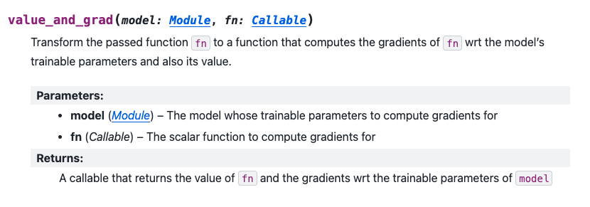
Which is wrapped by something that does not exist in Pytorch, which is the value_and_grad function in MLX:
self.__loss_function = nn.value_and_grad(
    self.__online_network,
    self.__loss_fn
)
The value_and_grad function is a wrapper that computes both the function and the gradient with respect to the inputs of the function. So it returns two values as stated in the documentation:
That’s it
Aaaaannnndd that’s it! The algorithm is not that complex.
The code is available here: https://github.com/Bornlex/MLX-DQN
References
- DeepMind DQN paper: https://storage.googleapis.com/deepmind-data/assets/papers/DeepMindNature14236Paper.pdf
- MLX documentation: https://ml-explore.github.io/mlx/build/html/index.html
- The code repository: https://github.com/Bornlex/MLX-DQN