The KV cache is an important feature in today’s LLM infrastructure. To understand exactly what it brings, let’s recall how LLMs are being used for inference.
Introduction
Feel free to read my article about Multi-head Self Attention for more explanation about the variations around the Attention layer !
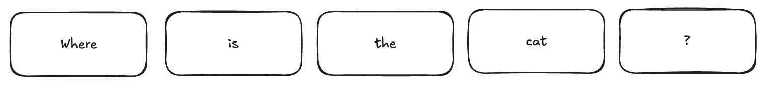
When LLMs are being used in production to generate text, they generate one word at a time. For example, from the following prompt :
Where is the cat ?
The model might generate something like :
The cat is sitting on the couch.
To make the visualisation simpler, we are going to make a few assumptions :
- the model uses words as tokens (which is not the case in reality)
- the batch is made of only one prompt (the one above)
- the embedding size $d$ is 3
- the attention dimension $d_k$ is the same as the embedding dimension $d$
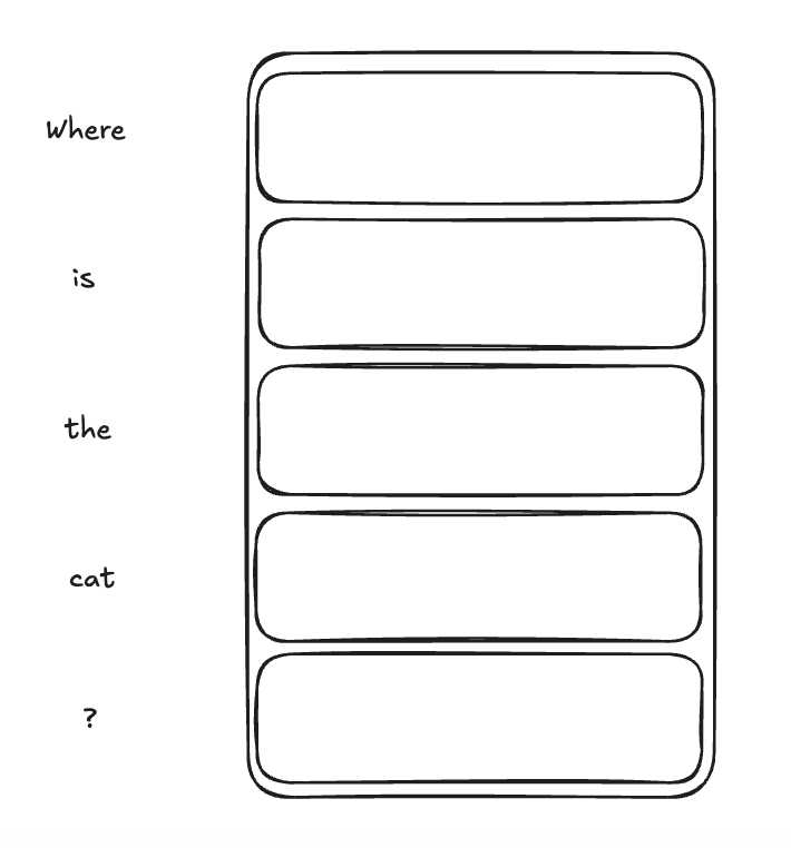
The prompt looks like this :
and once embedded, we get a tensor of the following shape (5, 3) :
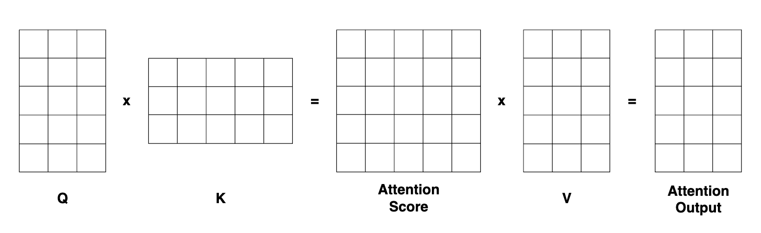
To start with the attention layer, we project this tensor along the queries, keys and values. Because we used $d = d_k$, the queries, keys and values tensors are going to have the same (5, 3) shape.
Then we need to compute the attention score by computing the matrix multiplication between the queries and the transposed keys. The result of this multiplication is a square matrix representing the attention score, mapping the input sequence tokens to themselves.
Every line I represented on the drawing is the mapping from one token of the input sequence to all the other tokens.
Let’s break down the operations :
- We first project the input sequence of shape by multiplying the input tensor with the 3 linear layers :
- The queries
- The keys
- The values
- We then compute the attention score
- We normalize it
- We multiply by the values
FLOPs
Let’s show what it looks like in terms of shapes and number of operations to perform :
| Shapes | # Operations | |
|---|---|---|
| Project the input in the queries space | (b, n, d) x (d, d) | b x n x d x dk |
| Project the input in the keys space | (b, n, d) x (d, d) | b x n x d x dk |
| Project the input in the values space | (b, n, d) x (d, d) | b x n x d x dk |
| Compute the attention score | (b, n, d) x (d, n) | b x n x dk x n |
| Normalize the attention score | (b, n, n) | b x n x n |
| Multiplication by the values | (b, n, n) x (n, d) | b x n x n x dv |
Which gives :
$$ 3 \times b \times n \times d \times d_k $$
To project the input tensor, then :
$$ b \times n^2 (d_k + d_v + 1) $$
For the rest of the calculation.
Note that the number of operations increases quadratically with the size of the input sequence.
Optimisation
On the first run, we have to compute the queries, keys and values for the whole sequence. Every token needs to be projected. Once we have the 3 matrices, we can compute the attention score, normalize it (by dividing by the dimension of the keys) and then apply softmax before finally multiplying this intermediary result by the values. We thus get the final result.
The final result will allow us to get the next predicted token, which here could be “The”, the first word answer by the model to our prompt.
Since LLMs are auto regressive models, this first prediction will be concatenated to the input sequence as the last token and the generation process will take place once again for the model to predict the second token. And so on until the model predicts an “end-of-text” token, indicating that the generation is over.
The second run interests us. Indeed, when we had the first sequence of tokens, we projected it by multiplying it by the queries, keys and values matrices and then we multiplied matrices together. It means that we already performed most of the needed computation for the second run.
We actually can simply multiply the new token by the weights matrices to have it projected, and then compute its attention score against the whole sequence to get the second predicted token.
Let’s show in red what we already computed from the previous run :
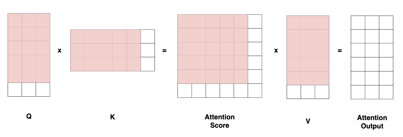
As we can see on the drawing, most of the projections and most of the attention score has already been computed from the previous run. Storing those values somewhere in cache is going to allow us to save a whole lot of processing time.
This is exactly what KV-cache is for.
Instead of recomputing the keys and values projections on the whole sequence, we are going to compute them on the latest token and concatenate it with the keys and values from the previous run that we stored in cache.
Last optimization
On top of this, note that we could only project only the last token in queries’ space. I have shown in blue the values required to compute the last vector in the attention layer’s output.
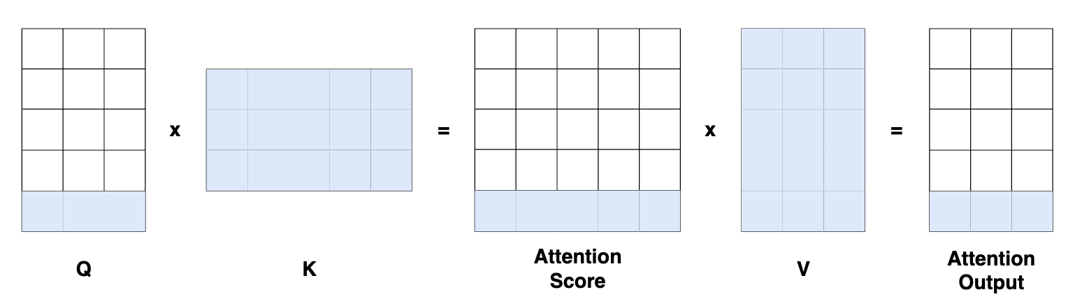
Since the prediction is going to be the last vector of the model, we need the full keys, the full values but only the last item of the queries projection.
Of course, if we stack attention layers, we are going to need to whole sequence, forcing us to compute the attention output on the whole sequence, and thus project the whole input sequence in queries space.
Implementation
The implementation is pretty straightforward. One can just register two buffers :
self.register_buffer("cache_k", None, persistent=False)
self.register_buffer("cache_v", None, persistent=False)
And then use them to retrieve the previous keys and values if they are in the cache already or simply fill the cache if they are not :
if use_cache:
    if self.cache_k is None:
        self.cache_k, self.cache_v = keys_new, values_new
    else:
        self.cache_k = torch.cat([self.cache_k, keys_new], dim=1)
        self.cache_v = torch.cat([self.cache_v, values_new], dim=1)
    keys, values = self.cache_k, self.cache_v
else:
    keys, values = keys_new, values_new
Important considerations
There can be some misconceptions about a few things regarding training, inference, masking, caching…
- Is KV-cache used for inference only ? Yes, KV-cache is used only for inference. During training, we need to build the computational graph so that we can backpropagate the gradient through the network to all the layers and update the weights.
- Why don’t we need to cache the queries ? We don’t need to cache the queries because during inference as opposed as during training, we only need to compute the queries on the very last token of the sequence. The context is stored already in the keys and values (which are cached). During training, we compute the queries on the whole sequence as a way of parallelizing the computation.
- Do we use masking during inference since we are only looking one token at a time ? Masking can be used during inference when input sequences inside a single batch do not have the same sizes. We could pad all sequences to the same length and then use a mask to zero out the corresponding padded tokens. A different approach would be to concatenate all the input sequences together, keep track of the boundaries and then keep the predicted tokens after after each sequence.