Shannon Entropy

Concept

In 1948, engineer and mathematician Claude Shannon published a foundational paper for computer science, and later artificial intelligence: A Mathematical Theory of Communication. This article defines a central idea in the training of current algorithms: information entropy.

$$ H = -\sum_{i = 1}^{n} p_i \log_2(p_i) $$

This formula allows us to quantify how random or organized a data source, such as a text-generating program, is. The higher the entropy, the more random the source; the lower the entropy, the more the data consists of recognizable patterns that allow us to predict the next words.

Let’s consider two examples:

1. The following sequence: 1010110010
2. And this one: 1111111011

These two sequences can represent successive coin tosses. 1 when the coin lands on heads, 0 when it lands on tails.

The first string appears random; it contains an equal number of 0s and 1s, making it difficult to predict the outcome of the next toss. The probability that the next visible side of the coin will be 1 or 0 is approximately 0.5.

The second string, however, contains almost all 1s, so we can reasonably assume that the next result will also be a 1, with a probability estimated at 90% based on the sequence.

In other words, we would have a lower chance of being wrong when trying to predict the second string compared to the first.

However, note that both sequences have an equal chance of occurring in reality: $p = \frac{1}{2^{10}}$.

Let’s calculate their entropies (using base-2 logarithm):

1. $H_1 = -\frac{1}{2} \log \frac{1}{2} - \frac{1}{2} \log \frac{1}{2} = - 2\log \frac{1}{2} = 1$
2. $H_2 = - \frac{1}{10} \log \frac{1}{10} - \frac{9}{10} \log \frac{9}{10} \sim - \frac{1}{10} \times -3.322 - \frac{9}{10} \times -0.152 = 0.469$

We observe that the entropy of the second string is lower than that of the first due to its less random nature.

Compression

The concept of entropy is closely related to the notion of compression. Indeed, if it is possible to predict the next symbol in a sequence of symbols, then it is possible to encode the most probable symbols using fewer bits. This way, the compressed message takes up less space, on average, than if all symbols had been encoded with the same number of bits.

This is known as entropy encoding. Various entropy encoding methods exist, the most well-known being Huffman coding and arithmetic coding, which are used, for example, in video and image compression.

Kolmogorov Complexity

In the 1960s, a Soviet mathematician, Andrey Kolmogorov, published what is now known as Kolmogorov complexity (or sometimes Kolmogorov-Solomonoff complexity), which is a measure of the difficulty of describing an object.

Remarkable Properties and Red-Painted Eggs

To illustrate, let’s take an example: imagine a series of simple objects, such as eggs, arranged in a grid (like a carton of square eggs).

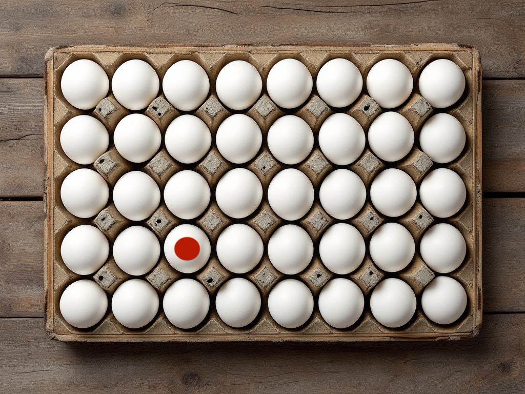
One egg is painted red.

If I wanted to indicate the red-painted egg, I would only need to say “the red-painted egg.” However, if I wanted to indicate any other egg, I would have no choice but to specify the row and column where it is located, as all other eggs are strictly identical.

The red-painted egg has a remarkable property: it is painted red.

This property makes it easy to describe compared to the others. Let’s quantify this difference:

• the red-painted egg
• the egg in the second row, fourth column

The first description takes 21 characters, while the second takes 45, more than twice as many. And we can note that the larger the egg carton, the more useful the remarkable property becomes. If I had to talk about the one thousand two hundred and seventeenth row, the second description would be even longer!

We can make the same observation with binary strings we mentioned earlier:

• 1010110010
• 1111111011

The first string does not have any apparent remarkable property, so the only way to describe it is to write it directly. However, the second string consists entirely of 1s except for the eighth bit, which is a zero.

Since the strings are short, the remarkable property doesn’t add much, but if the strings were made up of billions of bits, then describing the string would be much longer than saying it consists of 1s except for the eighth bit, which is constant.

This is what Kolmogorov complexity is about. In fact, we don’t use natural language (French, English, etc.) to talk about Kolmogorov complexity; instead, we use Turing machines, which are theoretical representations of algorithms.

Berry’s Paradox

Before discussing these algorithms, consider the following statement:

What is the smallest number that cannot be described in fewer than 1000 characters?

Well, this number is the smallest number that cannot be described in fewer than 1000 characters. However, this answer is fewer than 1000 characters. In other words, I can describe the smallest number that cannot be described in fewer than 1000 characters… in fewer than 1000 characters!

This is Berry’s paradox, which demonstrates the limitations of Kolmogorov complexity, at least as far as language is concerned.

Intuition Behind Kolmogorov Complexity Calculation

Let’s now consider algorithms to quantify Kolmogorov complexity. To keep it simple, we can even imagine using Python code. If we need to display a billion 1s on the screen, we can write the following code:

for _ in range(1000000000):
	print(1)

We notice something: if I want to write more 1s, for example, two billion instead of one billion, I only need to change what is inside the parentheses. The rest of the code can be reused.

Thus, we can denote the Kolmogorov complexity of this algorithm, which writes the digit 1 $n$ times on the screen, as:

$$ C(11…111) \le \log(n) + O(1) $$

Let’s break down this notation.

The $O(1)$ part corresponds to the portion of the algorithm that does not vary. We are not indicating here that it takes up one character in size; rather, we are indicating that it has nothing to do with the number of 1s we display. Whether there are 2 or millions of 1s, the size of this part of the code is constant, and that is what we indicate with this notation, which is pronounced “big O of 1” (the letter O).

The $\log(n)$ part corresponds to the number of 1s we want to display. The more 1s we want to display, the larger the number inside the parentheses becomes, but not linearly. For example, if I want to display the number 2 in binary, it is written as follows:

$$ 10 $$

which requires 2 characters. If I want to display 4 :

$$ 100 $$

which requires 3 characters. If I want to display 7 :

$$ 111 $$

which also requires 3 characters. We notice that $n$ written in binary increases logarithmically, in other words, we can calculate the number of bits needed to write a number $n$ by calculating $\log(n)$.

This is what this part of the code indicates.

The final point to clarify concerns the $\leq$ sign. This sign indicates that we cannot define Kolmogorov complexity precisely in an absolute manner because it depends on the language in which the algorithm is written. For example, this algorithm in Python:

for _ in range(1000000000):
	print(1)

does not take as many characters as this C code which is equivalent:

for (long i = 0 ; i < 1000000000 ; ++i)
{
	printf("1\n");
}

Of course, we are discussing here the complexity of the algorithm that displays 1s in a theoretical sense, not necessarily written in the programming languages we have available. This is why we cannot provide its exact complexity, but only an upper bound, hence the inequality in the formula.

Pi Compression

To conclude, and to make the connection with Shannon compression, let’s give an example of compression in the Kolmogorov sense.

We know that Pi’s decimals are random:

$$ \pi = 3.1415926535… $$

This means there is no relationship between the previous decimals and the following ones. If we wanted to compress $\pi$ using entropic coding, it would not be possible because all decimals have the same probability of appearing: $\frac{1}{10}$.

However, using Leibnitz’s formula:

$$ \pi = 4 \sum^{\infty}_{i = 0} \frac{(-1)^i}{2i + 1} $$

which when written in Python code gives:

def leibnitz_pi(n):
    pi_approx = 0
    
    for i in range(n):
        terme = (-1) ** i / (2 * i + 1)
        pi_approx += terme
    
    return 4 * pi_approx

The argument $n$ corresponds to the number of terms in the formula we want to calculate (roughly, how far $i$ will go in the sum). The more terms we add, the more precise the value of $\pi$ becomes.

Note that while this formula works, it converges slowly towards $\pi$. In practice, other algorithms are used to calculate the decimals of $\pi$. But this one is striking due to its very small size.

So if we want to compress $\pi$, rather than directly compressing its value, we can provide the algorithm that calculates it. We achieve remarkable compression here.

LLM

All this introduction for what? Well, to introduce an idea, rather a conceptual link that came to me recently, and that I would be pleased to formalize, share with readers, and subject to criticism, provided it is enlightened and constructive.

Language Model Training

Although there are various methods of training language models, the general procedure today follows two steps:

• pre-training
• post-training

These two phases aim for the same goal, making the model more performant, but are two distinct and complementary methods.

Pre-training

Anthropomorphically, pre-training corresponds to giving the model the basics of language.

From a more technical perspective, we reuse Claude Shannon’s idea that we discussed earlier and ask the model to predict the next token from a sequence of “tokens”.

To understand the general idea, the notion of token is not very important, we could replace token with word. Let’s just remember that a token is a fraction of a word of varying length, a rough rule is 4 tokens for 3 words, so a token counts for approximately 0.75 words.

We can find the formula used as the cost function during language model training in many papers, notably one of the first papers published by OpenAI: Improving Language Understanding by Generative Pre-Training. This is where we find the origin of the name GPT that we hear everywhere now.

Here is the formula:

$$ L(\mathcal{U}) = \sum_i \log p_{\theta}(u_i | u_{i - 1}…u_{i - k}) $$

In this formula, we find the following variables:

• $k$ the context size
• $\theta$ the model parameters
• $p$ the model itself, whose output is a probability distribution over all tokens

This formula is called the likelihood (or rather log-likelihood, due to the logarithm), it corresponds to the probability that the model correctly predicts certain words from the previous ones.

To calculate its value, we show $k$ tokens drawn from our dataset to the model, then ask it to predict the next one. But the actual next token is known, it’s simply the token that follows the sequence we drew. So we can verify if our model gave a high or low probability to this word, that’s the meaning of the part:

$$ p_{\theta}(u_i | u_{i - 1}…u_{i - k}) $$

This is the probability of seeing token $u_i$ given the previous tokens $u_{i - 1}, …, u_{i - k}$.

Note that the formula doesn’t use the probability directly, but rather the logarithm of the probability. Since a probability is between 0 and 1, the logarithm will have values between $\log(0) = -\infty$ and $\log(1) = 0$. The reason behind this choice is that it’s easier to handle large negative numbers than very small ones (probabilities can be very small).

The more the model gives a high probability to the current token appearing, the less it is “surprised” by the current token, the more performant it is.

We therefore seek to maximize this value.

During this pre-training phase, we monitor the evolution of the cost function value both on the training set and validation set, and when it’s sufficiently low and barely varies anymore, the pre-training is complete.

Post-training

Now that our model is capable of correctly predicting a word based on the previous ones and has a good understanding of language, it is possible to improve it further.

Indeed, for a model to be useful to users, it is often necessary for it to be able to respond to instructions or perform operations that require reasoning, not just complete a sentence or a piece of text.

To instill these new capabilities, the model can be improved in several ways, including:

• training it specifically to respond to instructions available in a dataset
• training it using reinforcement learning.

Within reinforcement learning, there are numerous methods:

• RLHF: reinforcement learning from human feedback
• PPO and its successor DPO: simpler methods to implement than RLHF that do not require developing specific models
• GRPO: a new method developed by the DeepSeek team

All these techniques are interesting but are not very important for the topic at hand. We can revisit them in a future article.

Connection Between Training and Shannon Entropy

We have seen that pre-training a model involves maximizing the log-likelihood. We notice that this log-likelihood formula somewhat resembles the formula for Shannon entropy.

Let’s discuss this resemblance.

As a reminder, here is the formula for log-likelihood:

$$ L(\mathcal{U}) = \sum_i \log p_{\theta}(u_i | u_{i - 1}…u_{i - k}) $$

The function $p_{\theta}(u_i | u_{i - 1}…u_{i - k})$ represents the probability that our model assigns to the token $u_i$ appearing, given the kk preceding tokens.

In practice, our model returns a probability distribution, meaning the probability for each token in the vocabulary to appear. This is a vector. If we consider the sentence “In my garage, there is my…” and we want to predict the word that follows this phrase, the context is composed of the words “in my garage, there is my,” and the model provides the probability of the next word:

$$ p_{\theta}(u_i) = \begin{bmatrix} p_{\theta}(\text{“dog”}) \ p_{\theta}(\text{“car”}) \ … \ p_{\theta}(\text{“plane”}) \end{bmatrix} $$

For all the words in the vocabulary (note that I am using words here, not tokens, simply to make the visualization more intuitive).

We know the current word, as it is the one that follows the sequence we passed to the model to predict the next one. The ground truth value (the actual word that follows the input sequence in the text), in this case, the word “car,” is also represented as a vector:

$$ q(u_i) = \begin{bmatrix} 0 \ 1 \ 0 \ 0 \ … \ 0 \end{bmatrix} $$

Here, the probability distribution qq is the true probability distribution, which we aim to approximate with our model.

It is a “one-hot” vector, meaning it has a 1 at the position of the word that is in the text and 0s at all other positions.

What we seek to maximize when adjusting our model’s parameters is the probability, according to our model, of predicting the correct word, in this case, “car.” We look at the probability that our model predicted for the word “car” to appear, which is simply:

$$ p_{\theta}(\text{“car”}) $$

When implementing this in a neural network, we actually compute the following:

$$ \prod_j^{d} p_{\theta}(u_i|u_{i-1},…,u_{i-k})_j^{q(u_i)_j} $$

This corresponds to multiplying together all the terms of the distribution given by the model, each raised to the power of the true probability value. This might seem strange at first, but it is actually quite simple and logical. Let’s calculate this result in our example:

Taking the logarithm:

We know that:

$$ \log a^b = b \log a $$

We then get:

We notice here that we have a formula very similar to the entropy formula. The difference between the entropy formula and this one is that the probability and the log of the probability are not calculated on the same distribution. This formula is known as cross-entropy (up to a negative sign).

Let’s complete the calculation.

The cross-entropy of our prediction for the word “car” is:

For all words that are not “car,” the probability according to the true distribution is 0. For the word “car,” it is 1, which simply gives us:

Finally:

And we perform this calculation for each word in the dataset.

Notice that this formula reaches a maximum value of 0 when our model assigns a probability of 1 to the correct word appearing, since $\log(1) = 0$.

Since optimization typically involves minimizing functions, we actually use the negative of this value, which we aim to minimize.

$$ \hat{\theta} = \argmin_{\theta} -L(\mathcal{U}) $$

Function calling

Gradually, we are getting to the heart of the article.

One aspect I find interesting about the use of language models today is what is known as “function calling.” This involves using models not to produce text, but to generate a sequence of external functions to be executed based on a user’s instructions. These functions can represent almost anything, such as:

• Querying a database
• Opening a webpage (as LLM interfaces like Mistral or OpenAI do when asked for information found on the internet)
• Changing a contact’s name in an address book

And much more.

In fact, we use language models as interfaces between a request stated in natural language and a sequence of operations necessary to fulfill it.

In other words, rather than producing the answer directly, we generate the program that provides the answer. Do you see where I’m going with this?

This way of functioning reminds me of Kolmogorov complexity. Suppose I ask an LLM to compile information from my database to answer a question. The LLM could provide the following sequence of operations:

1. Transform Julien’s request into a database query
2. Execute the database query
3. Compile the information
4. Format the information
5. Display the information on the screen

These operations are essentially a computer program written in a language where the basic operations are not those of assembly or Python, but high-level operations that interact with my system.

We can quantify the efficiency of the program returned by the LLM by simply counting the number of operations required to obtain the solution. This is somewhat akin to calculating its Kolmogorov complexity. The fewer operations the model needs to converge to the solution, the better it is.

The issue with using current language models is that they necessarily rely on language to provide this sequence of operations. Models used in “function calling” mode give responses like this:

[{
    "id": "call_12345xyz",
    "type": "function",
    "function": {
        "name": "get_weather",
        "arguments": "{\"location\":\"Paris, France\"}"
    }
}]

This response corresponds to calling the function get_weather with the argument location = Paris.

If multiple operations need to be chained together, they are listed in this format, one after the other.

However, this approach presents several challenges:

• The JSON format is rigid, and the output cannot be read if, for example, a parenthesis is missing.
• The number of tokens in the output used to call just one function is considerably high compared to what it could be if we had a vector of functions where we simply specified the ID.
• The sequence of operations is fixed. The LLM produces all the operations to be executed at once, without considering the intermediate outputs of the functions. It is not dynamic (although we could make successive calls so that the LLM only provides the next function to call, but then we would need to pass the entire context, which grows rapidly and could exceed the input size limit of the LLM quite quickly).

Number of tokens

Let’s evaluate the number of tokens required to produce the output:

from transformers import AutoTokenizer

string = '''
[{
    "id": "call_12345xyz",
    "type": "function",
    "function": {
        "name": "get_weather",
        "arguments": "{\"location\":\"Paris, France\"}"
    }
}]
'''

tokenizer = AutoTokenizer.from_pretrained('mistralai/Mistral-7B-Instruct-v0.3')
encoded = tokenizer.encode(string)

print(len(encoded))

This gives us the value 63. However, the information actually being transmitted is simply:

• The name of the function to call
• The argument to pass to the function

The function name to call is get_weather. Instead of directly providing the function name, the model could simply provide its index in a vector, similar to how it already handles tokens.

Regarding the argument, “Paris, France”, its size once encoded is only 4 tokens.

Thus, we could compress this output into 4 (the argument) + 1 (the function) = 5 tokens, representing a 92% compression compared to the initial 63 tokens.

Kolmogorov AI Framework

To formalize this idea, I would like to propose a framework for developing agents that are not merely LLMs to which successive calls are made.

Theoretically

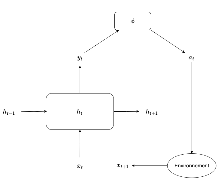
Execution Machine

We assume a machine capable of executing functions, which we denote as:

$$ \phi : \mathcal{X} \to \mathcal{Y} $$

Model

Let’s take the following recurrent state machine:

$$ \mathcal{A} := (H, h_0, \star, \bullet) $$

With:

• $H$ as the set of possible states of the machine (referencing the notation used for hidden states in RNNs)
• $h_0 \in H$ as the initial state of the machine
• $\star : H \times X \to H$ as the function that computes the new state from the current state and the current input
• $\bullet : H \to \mathcal{X}$ as the function that, given a state, provides the new instruction to execute along with its potential arguments
  • It is also possible to imagine this function providing a distribution over possible actions, which is then sampled to obtain the current action

The machine corresponds, in a way, to our programming language. The set of its instructions corresponds to the executable instructions, and the number of executions required to obtain the answer to a question corresponds to the Kolmogorov complexity of the program. This allows us to quantify the efficiency of the entire system.

Update after one instruction

To get $x_{t + 1}$, we compute $\phi(y_t)$ the following way:

$$ x_{t + 1} = (\phi \circ \bullet \circ \star)(h_t, x_t) = \phi(\bullet(\star(h_t, x_t))) $$

The cost function can be simply defined as the distance between the output of $\phi$ at time tt and the desired output.

From a theoretical standpoint, this framework has no limitations. One could easily imagine that $\phi$ corresponds to a processor, and the set of possible actions corresponds to the set of instructions for that processor (its assembly language, in a way). Thus, it is possible to generate all programs that can be executed on this processor.

In fact, any set of instructions from a Turing-complete language would suffice.

Process

For a simple stack-based language, the algorithm could work as follows:

1. The algorithm’s state is initialized to its starting value $h_0$.
2. A user enters an instruction in natural language.
3. This instruction is read by the model, which produces a vector $x_1$
4. The model updates its state $h_1 = \star(h_0, x_1)$.
5. The model calculates the current instruction $\hat{y}_1 = \bullet(h_1)$.
6. The execution machine executes the function $\phi(\hat{y}_1)$.
7. The result of the function is added to the stack so that it can be reused by subsequent functions.

Training

It seems to me that the best way to train a model of this type is by using reinforcement learning. Indeed, the need to perform a sequence of actions before obtaining a potential reward at the end of the sequence, based on whether the objective is achieved, intuitively resembles algorithms that can play chess by deducing the quality of intermediate moves from the outcome of the game.

The main theoretical difficulty arises from the fact that backpropagating the gradient through $\phi$ is complex, as this function is not differentiable.

I propose a training approach as illustrated in the diagram:

Reward

Considering we want to have an algorithm that is able to perform tasks as efficiently as possible, it gets the reward only if it achieves the task successfully.

Let us recall the Bellman equation for a Markov decision process:

$$ Q_{\pi}(s) = R(s, \pi(s)) + \gamma \sum_{s’} p(s’ | s, \pi(s)) Q_{\pi}(s’) $$

Considering sequences of maximum size $N$ (so the algorithm does not run indefinitely), we either get the reward for achieving the goal or we get cut if the program is not over after $N$ time steps:

$$ R(s_N) = \begin{cases} R -N \text{ if goal is reached} \ -N \text{ otherwise} \end{cases} $$

The term $-N$ comes from substracting 1 at every instruction run to force the model to perform its tasks as quick as possible.

Practicum

Scenario

Law enforcement, police, and intelligence services use all available information to carry out their missions.

Over the past few years, new valuable sources of information have emerged: blockchains.

Blockchains, the technologies supporting various cryptocurrencies, allow anonymous (or pseudonymous) users to conduct online transactions without intermediaries, outside the traditional (and regulated) financial system.

However, blockchains are complex tools, some of which are of considerable size and can be difficult for an agent or analyst to understand and analyze.

The scenario I propose to address is as follows: based on natural language commands, a language model will produce structured queries that can be used in a database specifically designed for storing graphs: Neo4j.

Questions that an investigator might ask include:

• What are the addresses to which address A has sent money?
• From which addresses has address A received money?
• What is the total amount sent by address A?
• Which addresses are involved in transaction T?
• How many outputs does transaction T have?
• What portion of the money received by address A comes from illegal sources?
• How many suspicious addresses are in the database?
• Are address A and address B connected?

Neo4j

Neo4j is a graph database that provides the following:

• Neo4j Aura: a managed database in the cloud
• Neo4j Desktop: a downloadable visualization interface
• Cypher: Neo4j’s language for querying the database

A Cypher query looks like this:

MATCH (a:Node {node_property: 'value'})-[:Relationship]->(t:Node2) RETURN t.property

We can observe keywords such as MATCH and RETURN, as well as node types (in parentheses) and relationship types between nodes (in brackets).

The previous query does the following:

• Returns the “property” property of all Node2 type nodes that are connected by the Relationship relation to the Node type node whose node_property equals “value”.

In our case, the Neo4j database will contain the following elements:

• Address nodes (Bitcoin addresses)
  • contain an address_id property
  • contain an address_type property whose values can be:
    • suspicious
    • legit
    • exchange
    • mixer
    • illegal
• Transaction nodes (transactions made by Bitcoin users)
  • contain a transaction_id property
• Input relationships (that connect addresses to transactions they participated in)
  • contain a value property (corresponding to what a given address put into the transaction)
• Output relationships (that connect transactions to recipient addresses)
  • contain a value property (corresponding to what an address received from the transaction)

In Neo4j Desktop, our database looks like this:

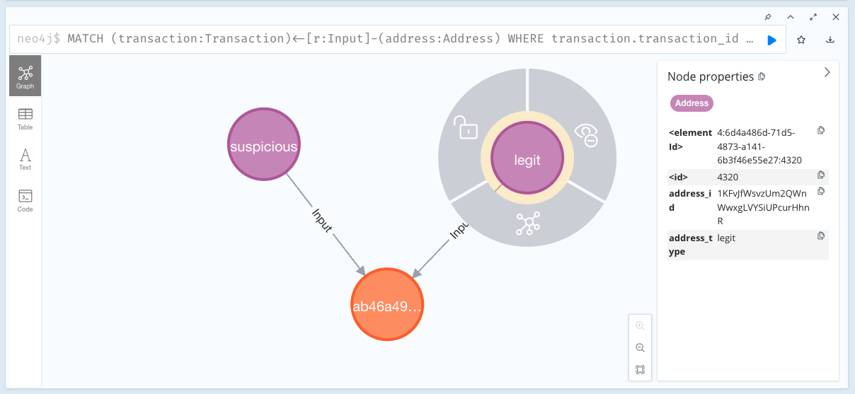
Here we can see an orange node that corresponds to a transaction. This node is connected to two other nodes, purple, which are the addresses. These two addresses put money into this transaction, which can be understood by the Input relationships going from the addresses to the transaction.

Functions

Here are some functions we could define and that our model could call:

• get_incoming_transactions
• get_outgoing_transactions
• get_input_addresses
• get_output_addresses
• get_inputs
• get_outputs
• get_address_type
• is_illegal
• sum
• count
• push

Along with a stack. Functions push their return value onto the stack and can pop one or more elements from the stack. For example:

• push → adds an element to the top of the stack, for example an address

• get_incoming_transactions → pops the element at the top of the stack (an address or list of addresses) and calls the get_incoming_transactions function passing this element as an argument, then adds the incoming transactions from the address in question to the top of the stack

  @with_driver
  def get_incoming_transactions(self, driver, address_id: str) -> list[str]:
      """
      :param driver: the neo4j driver
      :param address_id: the address hash
      :return: all incoming transactions
      """
      records, _, _ = driver.execute_query(
          'MATCH (address:Address)<-[r:Output]-(transaction:Transaction) '
          'WHERE address.address_id = $address_id '
          'RETURN transaction.transaction_id',
          address_id=address_id,
          routing_=RoutingControl.READ
      )
  
      return [record.value() for record in records]
  

• count → pops an element from the stack, calculates the size of the list and returns the result

The execution result is the element at the top of the stack.

Query Examples

Let’s take some examples:

1. To which addresses has address A sent money?
   1. push A
   2. get_outgoing_transactions
   3. get_output_addresses
2. From which addresses has address A received money?
   1. push A
   2. get_incoming_transactions
   3. get_input_addresses
3. What is the total amount sent by address A?
   1. push A
   2. get_outgoing_transactions
   3. sum
4. Which addresses are involved in transaction T?
   1. push T
   2. get_input_addresses
   3. push T
   4. get_output_addresses
   5. concat

Conclusion

The conceptual link I make with Kolmogorov complexity might be approximate, or seem distant, but I like it!

I find this idea of using LLMs as an interface for language but then having them use predefined functions rather than producing language refreshing.

I will develop an example using this framework, which I will post in the second part of this article, on my website.

References

• DeepSeek v3 Technical Report: https://arxiv.org/pdf/2412.19437
• Improving Language Understanding by Generative Pre-Training, OpenAI: https://cdn.openai.com/research-covers/language-unsupervised/language_understanding_paper.pdf
• A Mathematical Theory of Communication, Claude Shannon: https://people.math.harvard.edu/~ctm/home/text/others/shannon/entropy/entropy.pdf
• Andrei Kolmogorov’s Wikipedia page: https://fr.wikipedia.org/wiki/Andreï_Kolmogorov