Introduction
Transformers have revolutionized the field of machine learning, emerging as the dominant architectural choice across various applications.
However, their reliance on self-attention mechanisms introduces significant computational challenges, particularly due to quadratic time and memory complexity relative to sequence length.
While approximate solutions exist, their limited adoption stems from an overemphasis on theoretical FLOP counts rather than practical performance metrics.
In 2022, a paper introduced a way to compute the attention result by only working on sub vectors to reduce memory I/O.
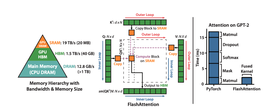
Hardware Performance
GPU memory
GPUs utilize two types of memory:
- High Bandwidth Memory (HBM)
- Static Random Access Memory (SRAM)
As comparison with a regular computer and CPU, SRAM can be seen as the registers of the GPU and HBM would be the RAM of the GPU.
While SRAM offers significantly faster processing speeds, it is considerably more limited in capacity compared to HBM. Due to the increasing speed gap between compute and memory operations, memory access has become a bottleneck, making efficient SRAM utilization increasingly critical for performance optimization.
Execution model
GPUs operate by utilizing a massive number of parallel threads to execute operations called kernels.
During execution, each kernel follows a specific pattern: it loads input data from the High Bandwidth Memory (HBM) into the faster Static Random Access Memory (SRAM), performs the necessary computations, and then writes the results back to HBM.
Performance characteristics
In analyzing the performance of deep learning operations, it’s helpful to distinguish between compute-bound and memory-bound behavior. Each operation can fall into one of these categories depending on whether computation or memory access is the primary bottleneck. A useful metric for identifying this is arithmetic intensity, defined as the number of arithmetic operations per byte of memory access. Higher arithmetic intensity typically indicates a compute-bound operation, while lower intensity points to a memory-bound one.
- Compute-bound operations:
- Performance is limited by the number of arithmetic operations.
- Memory access time is relatively small.
- Examples: matrix multiplication with a large inner dimension, convolution with a large number of channels.
- Memory-bound operations:
- Performance is limited by the number of memory accesses.
- Computation time is relatively small.
- Examples: elementwise operations (activation, dropout), reduction operations (sum, softmax, batch norm, layer norm).
Kernel fusion
If multiple times the same operation applied to the same input, the input is loaded only once from HBM instead of multiple times, which further reduces the number of operations.
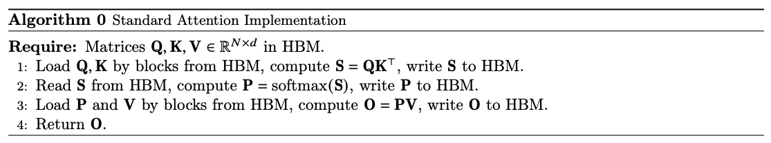
Standard Attention
Let’s take a look at how the attention mechanism works.
Given input sequences $Q, K, V \in \mathbb{R}^{N \times d}$, $N$ the sequence length and $d$ the head dimension, we want to compute the attention output $O \in \mathbb{R}^{N \times d}$:
$$ \textbf{S} = \textbf{QK}^T \in \mathbb{R}^{N \times N}, \textbf{P} = \text{softmax}(\textbf{S}) \in \mathbb{R}^{N \times N}, \textbf{O} = \textbf{PV} \in \mathbb{R}^{N \times d} $$Where softmax is applied row-wise.
Attention implementations creates matrices $\textbf{S, P}$ to HBM, which takes $O(N^2)$ memory.
Often $N \gg d$, for instance for GPT-2:
- $N = 1024$
- $d = 64$
Because the softmax is element-wise it is memory-bound.
There are other element-wise operations like masking and dropout. So there have been attempts to fuse operations like masking with softmax.
Here is the full algorithm, with the description of what is loaded from where and what is computed.
Flash Attention
The goal of FlashAttention is, given the input sequences $\textbf{Q, K, V} \in \mathbb{R}^{N \times d}$ in HBM, to compute the attention output $\textbf{O} \in \mathbb{R}^{N \times d}$ and write it to HBM. The goal is to reduce the amount of HBM accesses to sub-quadratic in $N$.
The strategy works as follow:
- Split the inputs $\textbf{Q, K, V}$ into blocks
- Load them from slow HBM to SRAM
- Compute the attention with respect to those blocks
- By scaling the output for each block by the right normalization factor before adding them up, we get the correct result at the end
Tiling
The idea of tiling is to compute attention by blocks. Unfortunately, the softmax couples the columns of $\textbf{K}$ (because one line of the $\textbf{P}$ matrix requires all the columns of the $\textbf{K}$ matrix to be computed, and the softmax needs them all at once).
So we need to decompose the large softmax with scaling.
As a reminder, the softmax function for vector $x \in \mathbb{R}^N$ is defined as follows:
$$ \text{softmax}(x_i) = \frac{e^{x_i}}{\sum_j^N e^{x_j}} \forall x_i \in x $$And can be rewritten as:
$$ \text{softmax}(x_i) = \frac{e^{x_i - m(x)}}{\sum_j^N e^{x_j - m(x)}} $$with $m(x) = \max_i x_i$.
The paper defines two function that are applied on vectors:
The function $f$ being defined as:
$$ f(x) = [e^{x_1 - m(x)}, ..., e^{x_B - m(x)}] $$And the function $l$:
$$ l(x) = \sum_i f(x)_i $$From those two functions, it is possible to compute the softmax of a vector by:
$$ \text{softmax}(x) = \frac{f(x)}{l(x)} $$Now imagine that the vector we want to compute the softmax on is big, and that we want to split it into two sub vectors.
Let’s take two vectors $x^{(1)}, x^{(2)} \in \mathbb{R}^B$ with $B$ being the size of a block. We can decompose the softmax of the concatenated vector $x = [x^{(1)}, x^{(2)}] \in \mathbb{R}^{2B}$ as:
$$ m(x) = m([x^{(1)}, x^{(2)}]) = m([m(x^{(1)}), m(x^{(2)})]) $$Where the global maximum is the maximum of local maxima, obviously.
Then the paper defines two local vectors:
- $f(x) = [e^{m(x^{(1)})-m(x)}f(x^{(1)}), e^{m(x^{(2)})-m(x)}f(x^{(2)})]$
- $l(x) = l([x^{(1)}, x^{(2)}])$
For a vector of size $B$.
When using this formula inside the $f$ vector above, we get for the first element of the vector:
$$ e^{x_1 - m(x^{(1)})} e^{m(x^{(1)}) - m(x)} = e^{x_1 - m(x)} $$Which is what we need to compute the softmax as seen in the softmax formula before.
The second term gives:
$$ l(x) = l([x^{(1)}, x^{(2)}]) = e^{m(x^{(1)}) - m(x)}l(x^{(1)}) + e^{m(x^{(2)}) - m(x)}l(x^{(2)}) $$Which indeed give the right softmax formula on the global vector after
$$ \text{softmax}(x) = \frac{f(x)}{l(x)} $$So by only keeping track of some local statistics like the maximum and the $l(x^{(i)})$ results, we can indeed compute the softmax function one block at a time.
Recomputation
The goal here is not to store the whole $\mathbf{S}, \mathbf{P} \in \mathbb{R}^{N \times N}$ matrices in memory.
Thanks to the method we described above, we can recompute the attention matrices $\mathbf{S}$ and $\mathbf{P}$ easily from both the softmax normalization statistics $(m, l)$ and the blocks of $\mathbf{Q}, \mathbf{K}, \mathbf{V}$ that are already loaded in SRAM.
Conclusion
The full algorithm (which is a bit complicated but explains precisely what to load to memory, what calculation to make, what to store…) and results can be found in the paper.
The idea of this article was more to understand how we can infer a global statistic about a matrix or a vector by only working on small pieces of such matrix or vector.
Sources
- Paper: https://arxiv.org/abs/2205.14135#
- Implementation: https://github.com/Dao-AILab/flash-attention