Context

Generating data is now a hot topic in machine learning. The idea of using statistical methods to produce synthetic data is rather old. Many methods are proven to be effective in different scenarios.

Today, the most well-known ways to generate synthetic data are:

VAE
GAN
Transformers

Transformers

A bit of history

We talked about RNN last week and we saw how they can be used to predict sequences. Unfortunately, RNN suffer some problems, especially with long sequences where they seem to forget what happened.

Also, training large models is complex. The higher the number of parameters the longer the inference time, and also the larger the required dataset. So a longer computation time for one prediction and more data to train big numbers of parameters. This is why we sometimes hear that deep learning was made possible by Nvidia and the CUDA library allowing researchers to train model on GPU, drastically reducing the time for one inference. Because the RNN is connected from the last prediction to the first, it is more difficult to parallelize training.

When predicting a sequence from a different sequence, the recurrent encoder-decoder appeared.

Later on some researchers introduced the concept of Attention in a paper that was later used by Google when creating the Transformer in the famous “Attention is all you need”.

This attention mechanism is at the very core of transformers, so let us talk about it. Attention uses a recurrent encoder-decoder framework and builds upon it a mechanism that allows the model to focus on specific parts of the input sequence.

Recurrent Encoder-Decoder

In the encoder-decoder framework, an recurrent encoder reads the input sequence, a sequence of vectors $x = (x_1, …, x_{d})$ into a vector $c$, called a hidden vector. From this hidden vector, a recurrent decoder decodes it into a different sequence.

The most common approach for the recurrent encoder is the one we discussed last week:

$$ h_t = f(x_t, h_{t - 1}) $$

And

$$ c = q(h_1, …, h_d) $$

Then the recurrent decoder is trained to predict the next vector based on the context vector and the previous tokens:

$$ p(y_t | y_1, …, y_{t - 1}, c) $$

Where in a RNN decoder, this probability is modeled as:

$$ g(y_{t - 1}, s_t, c) $$

Where $s_t$ is the hidden state of the recurrent decoder.

In a recurrent encoder-decoder, the first recurrent network encodes the whole sequence and passes it to the decode that decodes it into the output.

The architecture looks like this:

Encoder Decoder Architectre

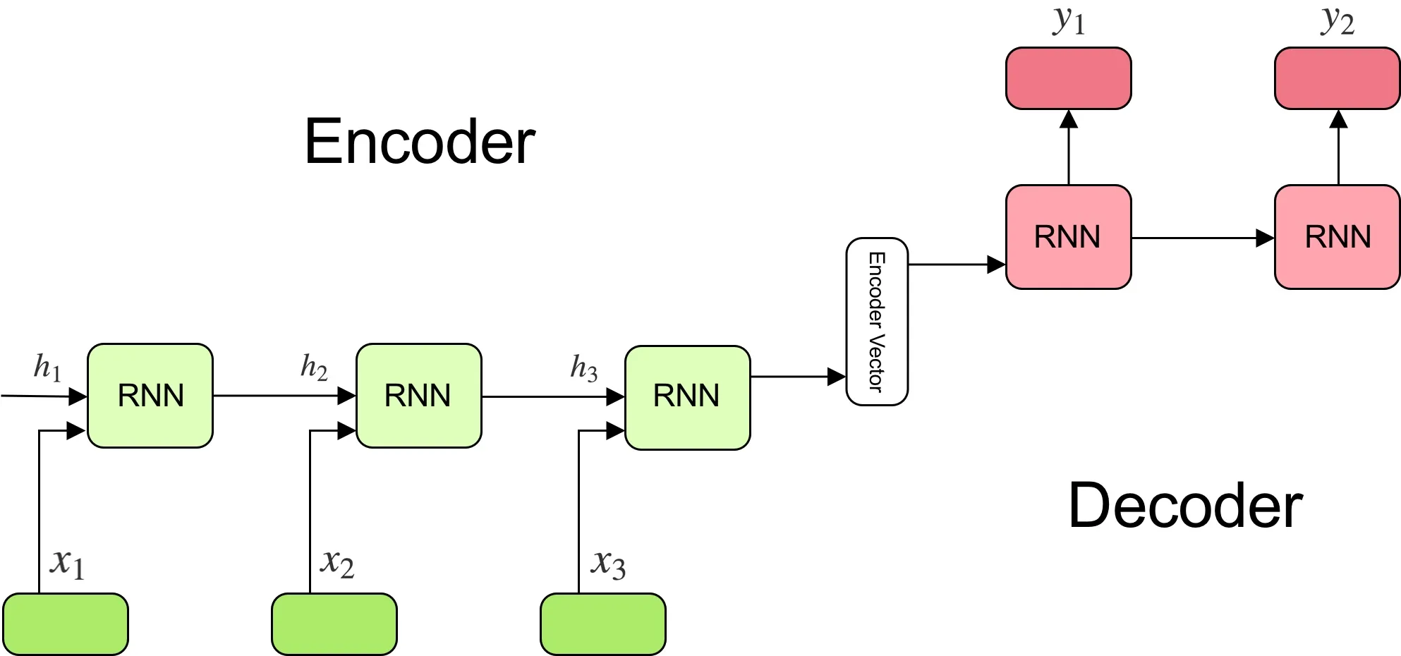
Note that sequences can be of different lengths.

Attention

Original attention mechanism

The attention mechanisms improves the previous framework by defining the conditional probability as:

$$ p(y_i | y_1, …, y_{i - 1}, x) = g(y_{i - 1}, s_i, c_i) $$

where $s_i$ is the hidden state at time $t$ computed by

$$ s_i = f(s_{i - 1}, y_{i - 1}, c_i) $$

The context vector depends on a sequence of annotations $(h_1, …, h_{d})$ to which an encoder maps the input into. Each annotation contains informations about the whole input sequence with a focus of the parts surrounding the i-th vector of the input sequence.

The context vector $c_i$ is computed as a weighted sum of annotations:

$$ c_i = \sum^{d}{j = 1} \alpha{ij} h_j $$

Where:

$$ \alpha_{ij} = \frac{\exp(e_{ij})}{\sum^d_{k = 1} \exp(e_{ik})} = \text{softmax}(e_{ij}) $$

Where:

$$ e_{ij} = a(s_{i - 1}, h_j) $$

Basically, it learns a matrix of values where the encoder hidden states are in rows and the decoder hidden states are in columns. This matrix is used to compute factors that will weight the encoder hidden states to give the model a more focused and relevant context.

The alignment is now learnt jointly with the encoder and the decoder.

Generalisation

The general attention mechanisms uses three main components:

the queries $Q$
the keys $K$
the values $V$

It gives:

$$ \text{attention}(Q, K, V) = \text{softmax}(\frac{QK^T}{\sqrt{d_k}}) V $$

Let us put this procedure into code to make it clearer.

First, start by defining the input of the attention layer. This could be for example the word embeddings.

word_1 = np.array([1, 0, 1, 0], dtype='float32')
word_2 = np.array([0, 2, 0, 2], dtype='float32')
word_3 = np.array([1, 1, 1, 1], dtype='float32')
words = np.vstack([word_1, word_2, word_3])

Obviously, this is going to be a (3, 4) numpy array.

Now let us define the weights of the attention layer:

wk = np.array([
	[0, 0, 1],
	[1, 1, 0],
	[0, 1, 0],
	[1, 1, 0]], dtype='float32'
)
wq = np.array([
	[1, 0, 1],
	[1, 0, 0],
	[0, 0, 1],
	[0, 1, 1]], dtype='float32'
)
wv = np.array([
	[0, 2, 0],
	[0, 3, 0],
	[1, 0, 3],
	[1, 1, 0]], dtype='float32'
)

The dimension of all the weights is: (4, 3).

Once we have the input vectors stacked together, we can compute the query representations, key representations and value representations. They are simply the dot products of the inputs and the weights:

query_representations = words @ wq
key_representations = words @ wk
value_representations = words @ wv

Each representation is a (3, 3) tensor.

And as a scaling factor, we also need the square root of the size of the representations:

dimension = float(query_representations.shape[0]) ** 0.5

Now that we have representations and the dimension, we can compute the attention scores:

attention_score = softmax(
	query_representations @ key_representations.T / dimension,
	axis=1
)

This is again a (3, 3) tensor.

And finally, let us compute the attention:

attention = attention_score @ value_representations

This is also a (3, 3) tensor.

We then need to propagate the gradients to the three different weight matrices:

$w_k \to \frac{\partial \text{attention score}}{\partial w_k}$
$w_q \to \frac{\partial \text{attention score}}{\partial w_q}$
$w_v \to \frac{\partial \text{attention score}}{\partial w_v}$

And this is how the Attention mechanism is trained.

Of course, many attention layers can be stacked together.

Tranformers

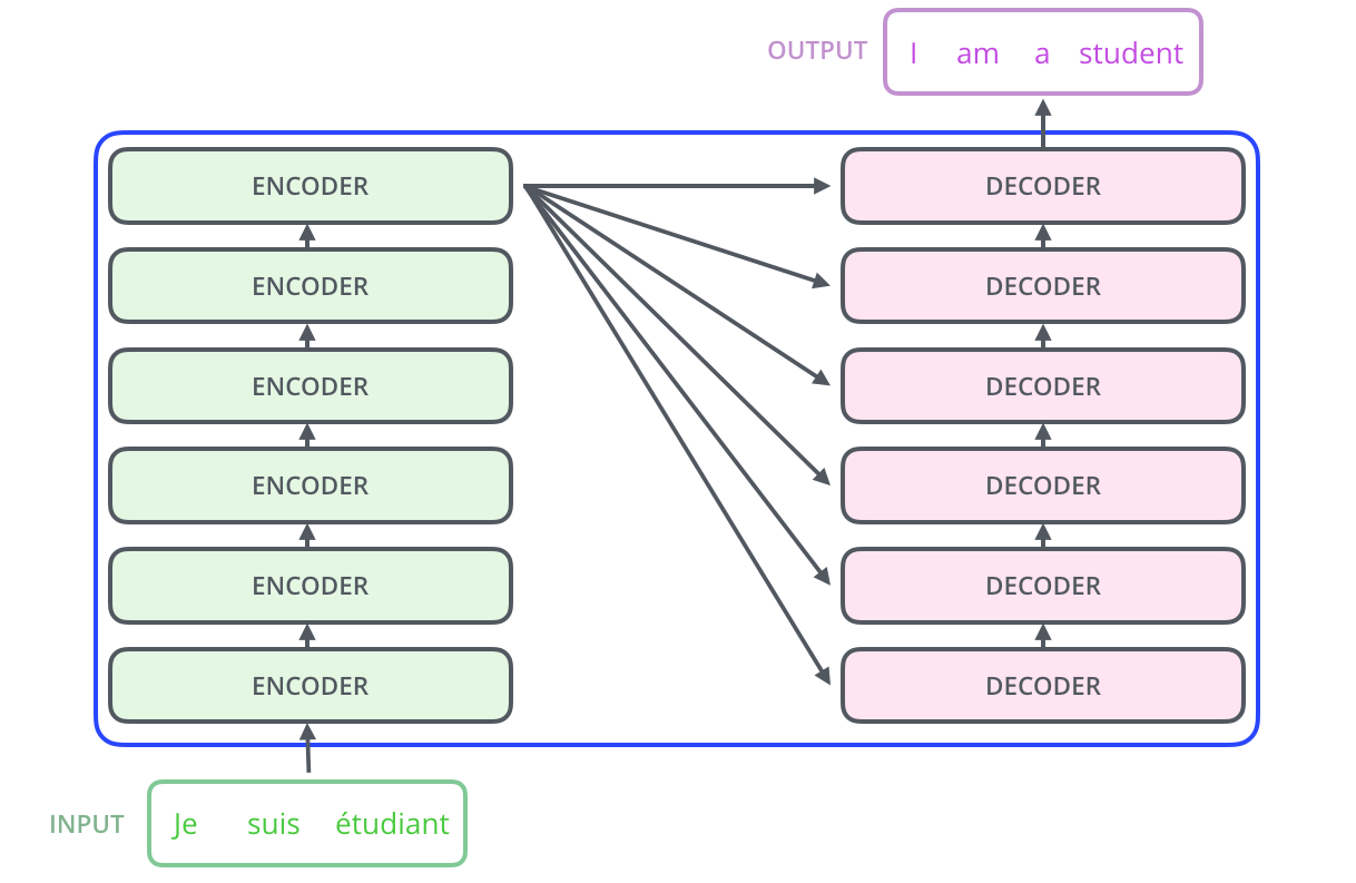
The Transformer architecture was first proposed in a paper called Attention is All You Need, by Google. It was intended for reducing the time to train sequence to sequence models.

Architecture

Its architecture is as follows:

Transformers

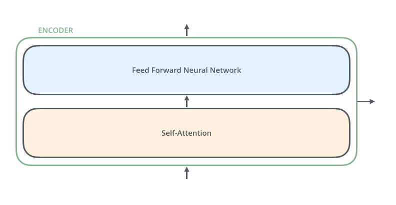
The encoders are made of two different layers:

A Self-Attention layer
A feed forward neural network

Encoder block

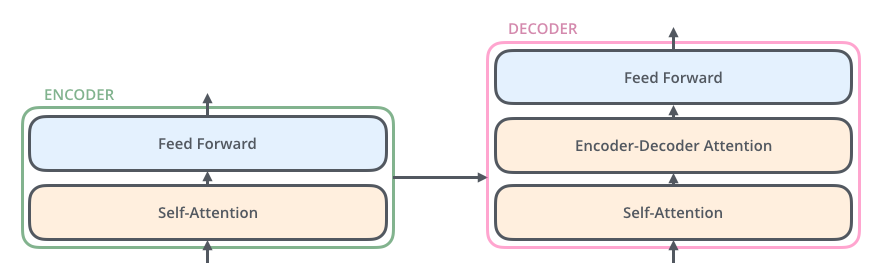
The decoders however are a bit more complicated because layers are also connected to the output of the last encoder:

Encoder Decoder

In the original paper, the number of levels (the number of encoders and the number of decoders) was set to 6. Of course, there is nothing magical about this number, one can experiment with different number.

Self-Attention

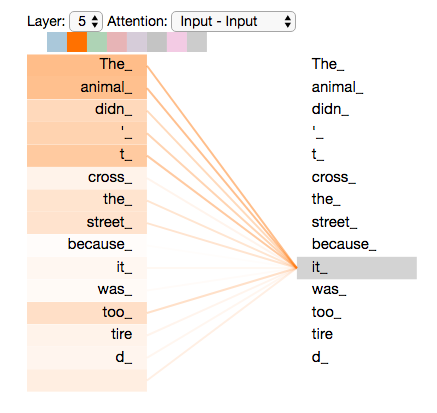
Self-Attention is conceptually very close to Attention. The difference is that Attention is looking at a first sequence to make predictions about a second sequence, Self-Attention is looking at the same sequence to make predictions.

It is used to model the links between elements inside sequences. Here is a quick example where we display how much a token from a sequence of words is related to other tokens inside the same sequence.

Attention

Multi-head Attention

Multi-head Attention refers to architectures where multiple Attention layers are stacked together.

Time Series

Now that we are familiar with the concept of Attention and Self-Attention, we would like to use those concepts to solve time series problems.

As we saw with the Attention mechanism and the code with it, we need to have vectors in order to compute the attention score. We need to embed our time series.

First, there are two kinds of input data:

univariate time series: one time series is used as input
multivariate time series: multiple time series are used as input data

Then there are several kinds of tasks:

classification
regression
forecasting
translation
segmentation

For translating or forecasting a time series, we want to predict future values of the time series based on its history. If we only need one value to be predicted, we can consider it as a sequence of size 1.

Practicum

In this exercise, we are going to develop a simple attention model using Pytorch, to predict a financial time series.

Data

The time series will be loaded from a csv file containing the Open High Low Close and Volume metrics for french CAC40 stock values.

The file can be downloaded here:

data.csv

We need to load the data and transform it to the right format.

def prepare_dataset(filename: str, n: int = 5) -> Tuple[np.ndarray, np.ndarray]:
    """
    Reads the file and prepares the dataset for training.
    The dataset consists of vectors of 5 elements: open, high, low, close, volume.
    An x is made n vectors of ohlcv values in the past and the y is the ohlcv value of the next day.

    xs: (batch, n, 5)
    ys: (batch, 5)

    :param filename: the data file to read
    :param n: the number of days to look back
    :return: tuple of xs and ys
    """
    pass

Here are the steps:

Read the file using pandas
Choosing a stock among the dataframe and filtering out other rows (for instance Accor)
Removing some useless columns: the first (that is unnamed), the date, the name
Replacing comas by dots inside the volume column
Removing rows containing nan
Casting values inside the dataframe as float32
Normalizing each column according to this formula: $x \leftarrow \frac{x - \mu(x)}{\sigma(x)}$
Return the data at the right numpy format:
1. xs: (n, 5) contains the n days before the prediction to be made
2. ys: (1, 5) contains the ground truth of the prediction

Forecasting model

The forecasting model will be made of two classes that inherits from nn.Module.

The first class will be implementing the Self Attention layer and the second class will be the model itself, containing a Self Attention layer as an attribute.

Self attention

class SelfAttention(nn.Module):
    def __init__(self, input_dim: int, output_dim: int):
        super().__init__()
        pass

    def forward(self, x: torch.Tensor):
        pass

Model

class TimeSeriesForecasting(nn.Module):
    def __init__(self, input_dim: int, hidden_dim: int, output_dim: int, sequence_length: int):
        super().__init__()
        pass

    def forward(self, x: torch.Tensor):
        pass

The model will contain a self attention layer along with a Flatten layer and a Linear layer.

Train procedure

Finally, the train procedure can be implemented. It should follow these steps:

Get the data
Split the dataset between train and test
Instantiate the model
Instantiate the criterion (MSE loss will work fine here)
Instantiate the optimizer
Train the model on batches (batch size of 8 works ok but feel free to experiment different batch sizes)
Test the model to display its predictions against the ground truth

OHLCV display

In order for you to see the results of your model’s predictions, here is a function that can be used:

def display_ohlc(targets: np.ndarray, predictions: np.ndarray):
    OPEN, HIGH, LOW, CLOSE, VOLUME = 0, 1, 2, 3, 4

    x = np.arange(0, targets.shape[0])
    fig, (ax, ax2) = plt.subplots(2, figsize=(12, 8), gridspec_kw={'height_ratios': [4, 1]})
    for i in range(targets.shape[0]):
        t_row = targets[i]
        p_row = predictions[i]
        target_color = '#228c45'
        predicted_color = '#4287f5'
        ax.plot([x[i], x[i]], [t_row[LOW], t_row[HIGH]], color=target_color)
        ax.plot([x[i], x[i] - 0.1], [t_row[OPEN], t_row[OPEN]], color=target_color)
        ax.plot([x[i], x[i] + 0.1], [t_row[CLOSE], t_row[CLOSE]], color=target_color)
        ax.plot([x[i], x[i]], [p_row[LOW], p_row[HIGH]], color=predicted_color)
        ax.plot([x[i], x[i] - 0.1], [p_row[OPEN], p_row[OPEN]], color=predicted_color)
        ax.plot([x[i], x[i] + 0.1], [p_row[CLOSE], p_row[CLOSE]], color=predicted_color)

    ax.spines['right'].set_visible(False)
    ax.spines['left'].set_visible(False)
    ax.spines['top'].set_visible(False)
    ax2.spines['right'].set_visible(False)
    ax2.spines['left'].set_visible(False)
    ax2.bar(x, targets[:, -1], color='lightgrey')

    ax.set_title('Time Series forecasting', loc='left', fontsize=20)
    plt.subplots_adjust(wspace=0, hspace=0)
    plt.show()

Results analysis

The predictions should be close to the ground truth. It might be interesting to see the attention scores of the predictions your algorithm will make. This should represent how much emphasis the model puts on each step in the past to make the prediction.

Do not hesitate to display attention scores as heatmaps. See if the attention scores are well balanced or not.

Sources

Neural Machine Translation by Jointly Learning to Align and Translate - https://arxiv.org/abs/1409.0473
Attention is All You Need - https://arxiv.org/abs/1706.03762
TimeGPT - https://arxiv.org/abs/2310.03589
Non-Stationary Transformers - https://github.com/thuml/Nonstationary_Transformers

Context#

Transformers#

A bit of history#

Recurrent Encoder-Decoder#

Attention#

Original attention mechanism#

Generalisation#

Tranformers#

Architecture#

Self-Attention#

Multi-head Attention#

Time Series#

Practicum#

Data#

Forecasting model#

Self attention#

Model#

Train procedure#

OHLCV display#

Results analysis#

Sources#

Context

Transformers

A bit of history

Recurrent Encoder-Decoder

Attention

Original attention mechanism

Generalisation

Tranformers

Architecture

Self-Attention

Multi-head Attention

Time Series

Practicum

Data

Forecasting model

Self attention

Model

Train procedure

OHLCV display

Results analysis

Sources