Introduction

Motivation

Why is it necessary to introduce the concept of recurrence in neural networks?

We know certain things in sequence. Let’s take the example of the alphabet. We can recite it without even thinking about it in the order from A to Z. However, if we were asked to recite it backwards, or even worse, to recite the alphabet based on the position of the letters (give the 17th letter, then the 5th…), we would be unable to do so.

We would be unable to do so because when we learned it, we always heard it in order. Our brain recorded the pairs of letters that follow each other. In a way, the clue to know the next letter is located in the previous one.

This is exactly the idea behind recurrent networks that we are going to talk about today.

Let’s take a second example: the trajectory of a ball.

If we are trying to build an algorithm that can give us the trajectory of a bouncing ball, for example, knowing the position of the ball at a given time $t$ is not enough. We also need to know its velocity. And its velocity is nothing more than the difference between its current position and its previous position. In other words, it is necessary to store in memory the information of previous positions in order to make a future prediction.

Intuition

A recurrent neural network operates on the following principle:

Recurrent Neural Principle

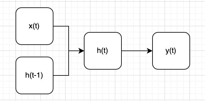
At each step, the network builds a hidden state $h_t$ using current input $x_t$ and previous hidden state $h_{t-1}$. Once this state is constructed, the network uses it to make a prediction $y_t$.

Let us not that the hidden state update equation can be written like a stochastic process one.

$h_t = f(h_{t-1}, x_t)$

In the simplest case, considering linear activation function :

$h_t = h_{t-1} + x_t$ qui ressemble à la marche aléatoire.

Question

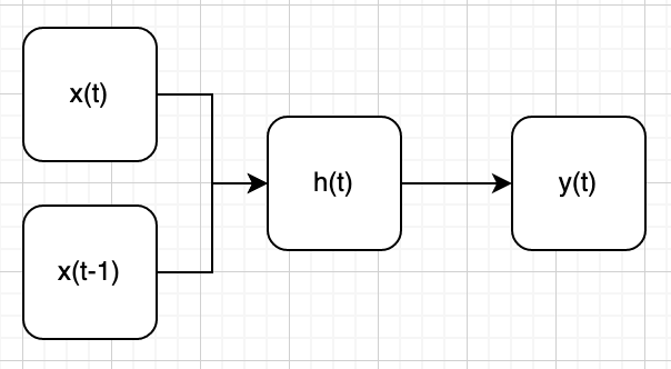
Why is the following architecture not as expressive as the previous one?

Less expressive RNN

Answer

Let’s write three iterations of the calculation using the following architecture:

in0 + in1 → hidden1 → output1
in1 + in2 → hidden2 → output2
in2 + in3 → hidden3 → output3

Let’s assign colors to the entries and see what information the hidden state preserves at each step:

in0 + in1 → hidden1 → output1
in1 + in2 → hidden2 → output2
in2 + in3 → hidden3 → output3

It can be observed that hidden state 3 no longer contains any information related to input 0 or input 1. Because the hidden state at time step $t$ is not used in the construction of the hidden state at time step $t+1$, the information it contained is completely lost.

Here we note a fundamental difference with a game like chess, for example, which does not require memory. The current input provides all the necessary information to determine the best move.

Types of RNN

There are multiple types of recurrent neural networks:

Types of RNN

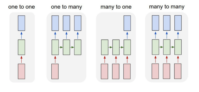
Let us give a few examples :

One-to-many : image annotation
Many-to-one : time series classification, text classification
Many-to-many : translation, segmentation, video classification

Backward Propagation

Now that we are familiar with the recurrent neural network architecture, we need to understand how to update the weights in order to train the model. Let us consider the following recurrent network:

Backpropagation through time

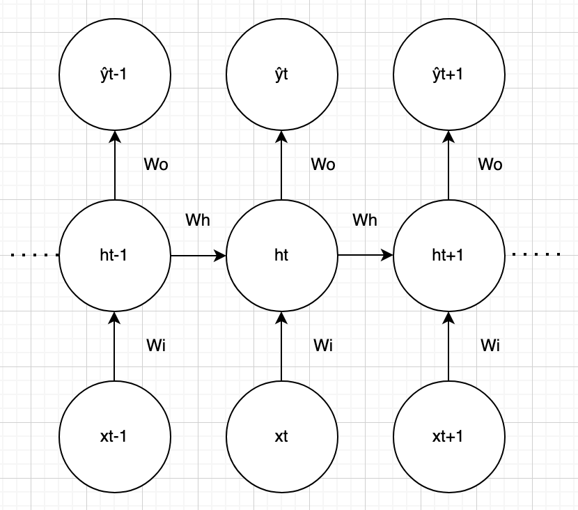
And the following notations:

$\hat{y}_t = f(o_t)$ the prediction, with $f = \sigma$ the sigmoid activation function
$o_t = w_o h_t$
$h_t = g(a_t)$ with $g = \sigma$
$a_t = w_h h_{t - 1} + w_i x_t$
$y_t$ the ground truth

We want to be able to compute the gradient of the weights of the model:

$w_o$ : output weights
$w_h$ : hidden weights
$w_i$ : input weights

Let us consider an arbitrary loss $L : (y_1, y_2) \mapsto l \in \mathbb{R}$.

The value of the overall loss is the sum of all the predictions:

$$ L = \sum_N^t L_t = \sum_N^t L(\hat{y}_t, y_t) $$

And:

$$ L_t = (\hat{y}_t - y_t)^2 $$

We want the expressions of:

$\frac{\partial L}{\partial w_o}$
$\frac{\partial L}{\partial w_h}$
$\frac{\partial L}{\partial w_i}$

We will need the derivative of the activation function:

$$ \sigma’(x) = \sigma(x)(1 - \sigma(x)) $$

Quick note

One can observe that the weights of the network are shared among all predictions. Because of this very specific property, it is hard to give an expression for the gradients of the weights.

To solve this, we are going to consider a time version of the weights: $w_{ot}$ which is the value of $w_o$ at step $t$.

Now that we have a version of our weight that appears only at step $t$, it is much easier to give the expression of its gradient.

In order to take into account all the prediction steps, we will compute those gradients at each time $t$.

1. Gradient with respect to $o_t$ : $\frac{\partial L}{\partial o_t}$

In order to compute all the expressions we need, we are going to have to compute two expressions first. They appear in most of the expressions of the gradient.

The first one is:

$$ \frac{\partial L}{\partial o_t} = \sum_i^n \frac{\partial L_i}{\partial o_t} = \frac{\partial L_t}{\partial o_t} = \frac{\partial L_t}{\partial \hat{y_t}} \frac{\partial \hat{y_t}}{\partial o_t} = 2(\hat{y}_t - y_t) . \hat{y_t}(1 - \hat{y_t}) $$

2. Gradient wrt $h_t$ : $\frac{\partial L}{\partial h_t}$

$$ \frac{\partial L}{\partial h_t} = \frac{\partial L_t}{\partial h_t} + \frac{\partial L_{i > t}}{\partial h_t} = \frac{\partial L_t}{\partial o_t}.\frac{\partial o_t}{\partial h_t} + \frac{\partial L}{\partial h_{t+1}}.\frac{\partial h_{t+1}}{\partial a_{t+1}}.\frac{\partial a_{t+1}}{\partial h_t} $$

$$ \frac{\partial L}{\partial h_t} = w_o\frac{\partial L_t}{\partial o_t} + w_h h_{t+1}(1 - h_{t+1})\frac{\partial L}{\partial h_{t+1}} $$

Notice how we get a recursive expression for this gradient. Practically we will compute it from the very last prediction of the sequence where $\frac{\delta L}{\delta h_{t + 1}} = 0$ and for all other prediction by keeping the previous value of the gradient with respect to the hidden state.

3. Gradient wrt $w_o$ : $\frac{\partial L}{\partial w_o}$

The easiest expression to compute is the gradient with respect to $w_o$ because it only affects the prediction at time $t$.

$$ \frac{\partial L}{\partial y_t} = \frac{\partial }{\partial y_t} \sum_N^t L_t = \frac{\partial}{\partial y_t} L_t = L_t’(y_t) $$

$$ \frac{\partial L}{\partial w_o} = \frac{\partial L_t}{\partial o_t} . \frac{\partial o_t}{\partial w_o} = \frac{\partial L}{\partial o_t}h_t $$

The term $\frac{\partial L}{\partial o_t}$ is already known from 1.

4. Gradient wrt $w_i$ : $\frac{\partial L}{\partial w_i}$

Because $w_i$ affects the hidden state at time $t$, it affects prediction at time $t$ but also later predictions.

$$ \frac{\partial L}{\partial w_i} = \frac{\partial L}{\partial h_t}\frac{\partial h_t}{\partial a_t}\frac{\partial a_t}{\partial w_i} = \frac{\partial L}{\partial h_t}h_t(1-h_t)x_t $$

The term $\frac{\partial L}{\partial h_t}$ is already known from 2.

5. Gradient wrt $w_h$ : $\frac{\partial L}{\partial w_h}$

Finally:

$$ \frac{\partial L}{\partial w_h} = \frac{\partial L}{\partial h_t} . \frac{\partial h_t}{\partial a_t}.\frac{\partial a_t}{\partial w_h} = h_{t-1}h_t(1 - h_t)\frac{\partial L}{\partial h_t} $$

Again the term $\frac{\partial L}{\partial h_t}$ is already known from 2.

Relationship between RNN and ARMA models

A question should be asked: why do we need recurrent neural network?

Of course, we answered it intuitively at the beginning of this lecture. But can we answer theoretically?

Can we show where recurrent neural networks are better models that regular neural networks?

Let us remember the traditional approach to time series forecasting: the ARMA(p, q) model.

$$ x_t = \sum^p_{i = 1} \phi_i x_{i - 1} + \sum^q_{j = 1} \theta_i e_{i - 1} + e_t $$

And now let us show the equation of the hidden state of a simple RNN with no activation function:

$$ h_t = a h_{t - 1} + bx_t $$

Which recursively gives:

$$ h_t = a^p h_{t - p} + \sum^p_{i = 0} \phi_i x_{t - i} $$

Considering that the first values of the hidden state is a constant, we might have:

$$ h_t = c + \sum^p_{i = 0} \phi_i x_{t - i} $$

Which is the equation of a moving average model of order p.

Appendix

Jacobian Matrix

TP : RNN for Binary Sum

Context

We aim at writing a simple RNN that will be able to sum two binary strings.

Inputs will be successive bits that the network will have to add and the output is going to be the result bit.

In such a case, we obviously see why a RNN might work where a simple NN could not, because of the result of the previous addition needs to be kept in memory.

$\begin{matrix} & 1 & 0 & 1 & 1 \

& 0 & 0 & 0 & 1 \ = & 1 & 1 & 0 & 0 \ \end{matrix}$

Link

Google Colaboratory

Correction

get_sample

def get_sample(dataset):
    largest_number = max(dataset.keys())
    while True:
        a = np.random.randint(largest_number)
        b = np.random.randint(largest_number)
        c = a + b
        if c <= largest_number:
            return dataset[a], dataset[b], dataset[c]

init_nn

def init_nn(inp_dim, hid_dim, out_dim):
    inp_layer = 2 * np.random.random((inp_dim, hid_dim)) - 1
    hid_layer = 2 * np.random.random((hid_dim, hid_dim)) - 1
    out_layer = 2 * np.random.random((hid_dim, out_dim)) - 1
    return inp_layer, hid_layer, out_layer

train

def train(
    wi: np.ndarray,
    wh: np.ndarray,
    wo: np.ndarray,
    iterations: int,
    dataset: tuple,
    hidden_dimension
):
    for iteration in range(iterations):
        wi_update = np.zeros_like(wi)
        wh_update = np.zeros_like(wh)
        wo_update = np.zeros_like(wo)

        a, b, c = get_sample(dataset)
        d = np.zeros_like(c)
        number_bits = len(c)

        error = 0
        o_deltas = list()
        ht_values = list()
        ht_values.append(np.zeros((1, hidden_dimension)))
        for pos in range(number_bits):
            index = number_bits - pos - 1
            x = np.array([[a[index], b[index]]])
            y = np.array([[c[index]]])

            at = x @ wi + ht_values[-1] @ wh
            ht = sigmoid(at)
            ot = ht @ wo
            yt = sigmoid(ot)

            prediction_error = 2 * (yt - y)
            o_deltas.append(prediction_error * yt * (1 - yt))
            error += np.abs(prediction_error[0])

            d[index] = np.round(yt[0][0])
            ht_values.append(copy.deepcopy(ht))

        future_ht_delta = np.zeros_like(ht_values[-1])
        for i in range(number_bits):
            x = np.array([[a[i], b[i]]])
            ht = ht_values[-i - 1]
            prev_ht = ht_values[-i - 2]
            o_delta = o_deltas[-i - 1]

            ht_delta = np.clip(
                (o_delta @ wo.T + future_ht_delta @ wh.T) * (ht * (1 - ht)),
                -5, 5
            )

            wo_update += (o_delta @ ht).T
            wh_update += prev_ht * ht * (1 - ht) * ht_delta
            wi_update += x.T @ (ht * (1 - ht) * ht_delta)

            future_ht_delta = copy.deepcopy(ht_delta)

        wi -= wi_update * alpha
        wh -= wh_update * alpha
        wo -= wo_update * alpha

        if iteration % 1000 == 0:
            print(f"[{iteration}|{iterations}] Error: {error}")
            print(f"\tTrue: {c} = {a} + {b}")
            print(f"\tPred: {d}")

Introduction#

Motivation#

Intuition#

Question#

Answer#

Types of RNN#

Backward Propagation#

Quick note#

1. Gradient with respect to $o_t$ : $\frac{\partial L}{\partial o_t}$#

2. Gradient wrt $h_t$ : $\frac{\partial L}{\partial h_t}$#

3. Gradient wrt $w_o$ : $\frac{\partial L}{\partial w_o}$#

4. Gradient wrt $w_i$ : $\frac{\partial L}{\partial w_i}$#

5. Gradient wrt $w_h$ : $\frac{\partial L}{\partial w_h}$#

Relationship between RNN and ARMA models#

Appendix#

Jacobian Matrix#

TP : RNN for Binary Sum#

Context#

Link#

Correction#

get_sample#

init_nn#

train#

Introduction

Motivation

Intuition

Question

Answer

Types of RNN

Backward Propagation

Quick note

1. Gradient with respect to $o_t$ : $\frac{\partial L}{\partial o_t}$

2. Gradient wrt $h_t$ : $\frac{\partial L}{\partial h_t}$

3. Gradient wrt $w_o$ : $\frac{\partial L}{\partial w_o}$

4. Gradient wrt $w_i$ : $\frac{\partial L}{\partial w_i}$

5. Gradient wrt $w_h$ : $\frac{\partial L}{\partial w_h}$

Relationship between RNN and ARMA models

Appendix

Jacobian Matrix

TP : RNN for Binary Sum

Context

Link

Correction

get_sample

init_nn

train