Time Series
Time series & stochastic processes
A time series is a set of observations $x_t$ generated sequentially over time $t$.
There are two main types of time series:
- continuous time series
- discrete time series
We can also differentiate time series whose values can be determined by mathematical functions, deterministic time series, from the time series that have some random component, non-deterministic time series.
To forecast non-deterministic time series, we assume that there is a probability model that generates the observations of the time series.
Definition: A discrete time stochastic process is a sequence of random variables $ \left\{ X_t \right\} $ defined over time $t$.
We can then think about a time series as a particular realization of a stochastic process: $ (X_0, X_1, …, X_n) $.
Time series analysis is about uncovering the stochastic process that has generated the time series.
Stationarity
When forecasting, we assume that some properties of the time series are maintained over time. For example, if a time series tend to increase or if the observations are always around the same value, we expect this characteristics to be present on future observations.
Let’s define these properties and the time series whose properties are constant over time.
Let $\left\{ X_t \right\}$ be a time series. The mean function of $\left\{ X_t \right\}$ is defined as
$$ \mu(t) = E(X_t) $$
where $E(X_t)$ is the expected value of the random variable $X_t$.
Now, let’s define the covariance function between two random variables of our time series.
Let $\left\{ X_t \right\}$ be a time series. The covariance function of $\left\{ X_t \right\}$ is
$$ \gamma(t, t+h) = \text{Cov}(X_t, X_{t+h}) = E[(X_t - \mu(t)). (X_{t+h} - \mu(t + h))] $$
Where $t = 1, 2, …, n$ and $h = 1, 2, …, n - t$.
Let $\left\{ X_t \right\}$ be a time series. $\left\{ X_t \right\}$ is strictly stationary if $(X_1, …, X_n)$ and $(X_{1 + h}, …, X_{n + h})$ have the same joint distribution for all $h$.
It means that the time series is stationary if the distribution is unchanged after any arbitrary shift.
Let $\left|{ X_t \right\}$ be a time series. $\left\{ X_t \right\}$ is weakly stationary if
- $E(X_t^2) < \infty$ for all $t$
- $\mu(r) = \mu(s)$ for all $r, s$
- $\gamma(r, r + h) = \gamma(s, s + h)$ for all $r, s, h$
In other words, a time series is weakly stationary if its second moment is always finite, its mean is constant and its covariance depends only on the distance between observations, also called lag.
From now on, when talking about stationarity, we will mean weakly stationarity.
Correlation
Since the covariance only depends on lag $h$ on weakly stationary time series, we can define the covariance function of these time series with only variable. This function is known as autocovariance function.
Let $\left\{ X_t \right\}$ be a weakly stationary time series. The autocovariance function of $\left\{ X_t \right\}$ at lag $h$ is
$$ \gamma(h) = \text{Cov}(X_t, X_{t + h}) = E[(X_t - \mu) . (X_{t + h} - \mu)] $$
One can notice that $\gamma(0) = E[(X_t - \mu)^2] = \sigma^2$ is the variance of the time series.
From this definition, we can define the autocorrelation function.
Let $\left\{ X_t \right\}$ be a weakly stationary time series. The autocorrelation function of $\left\{ X_t \right\}$ at lag $h$ is
$$ \rho(h) = \frac{\gamma(h)}{\gamma(0)} $$
We easily see that $\rho(0) = 1$. Also, we can notice that $|\rho(h)| \leq 1$ because of the Cauchy-Schwarz inequality:
$$ |\gamma(h)|^2 = (E[(X_t - \mu) . (X_{t + h} - \mu)])^2 \leq E[(X_t - \mu)^2] . E[(X_{t + h} - \mu)^2] = \gamma(0)^2 $$
Proof
Analyse of the $\lambda \mapsto E[(\lambda X - Y)^2]$ polynom.
Examples
Now that we gave some definitions, let’s show some examples of time series and their characteristics.
White noise
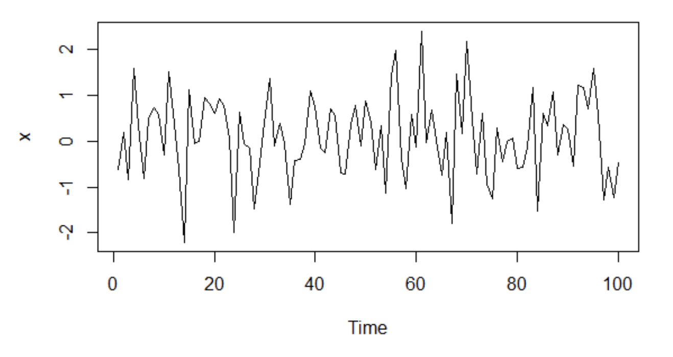
White noise consists of a sequence of uncorrelated random variables $\left\{ X_t \right\}$ with mean $\mu$ and variance $\sigma^2$. If the random variables follow a normal distribution, the series is called gaussian white noise. Gaussian white noise is made of independent and identically distributed variables.
Here is a plot of the gaussian white noise of variance
$\sigma^2 = 1$ and $\mu = 0$.
Since the random variables are independent, they are not correlated, so its autocovariance function is $\sigma^2$ at lag $0$ and $0$ at lag $h > 0$. Its autocorrelation is $1$ at lag $0$ and $0$ at lag $h > 0$.
Random walk
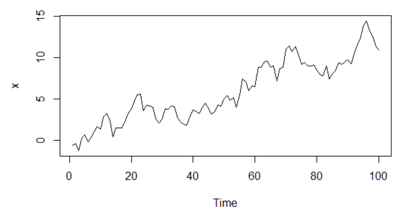
Definition: Let $\left\{ X_t \right\}$ be a time series and $\left\{ W_t \right\}$ an IID noise time series. $\left\{ X_t \right\}$ is a random walk if
- $X_1 = W_1$
- $X_t = X_{t-1} + W_t$ if $t > 1$
Note that a random walk can also be written as
$$ X_t = \sum^t_{i=1} W_i $$
The mean of this time series is the mean of $\left\{ W_t \right\}$ and its covariance is given by :
$$ \text{Cov}(X_t, X_{t + h}) = \text{Cov}(\sum^t_{i=1} W_i, \sum^{t+h}_{i=1} W_i) = \sum^t_{i=1} \text{Cov}(W_i, W_i) = t \sigma^2 $$
Exercise: prove the previous result
$$ \text{Cov}(X_t, X_{t + h}) = \text{Cov}(\sum^t_{i=1} W_i, \sum^{t+h}_{i=1} W_i) $$
$$ \text{Cov}(X_t, X_{t + h}) = \text{Cov}(\sum^t_{i=1} W_i, \sum^{t}_{i=1} W_i + \sum^{t + h}_{i=t + 1} W_i) $$
$$ \text{Cov}(X_t, X_{t + h}) = \text{Cov}(\sum^t_{i=1} W_i, \sum^{t}_{i=1} W_i) + \text{Cov}(\sum^t_{i=1} W_i, \sum^{t + h}_{i=t + 1} W_i) $$
$$ \text{Cov}(X_t, X_{t + h}) = \text{Var}(X_t) + 0 $$
$$ \text{Cov}(X_t, X_{t + h}) = \sum_i^t\text{Var}(W_i) $$
Because $W_i$ are IID.
$$ \text{Cov}(X_t, X_{t + h}) = t \sigma^2 $$
Because the covariance function depends on $t$, the process is not stationary.
Quarterly earnings
Finally, let’s give an example of real data. The time series of quarterly earnings in US dollars per Johnson & Johnson share.
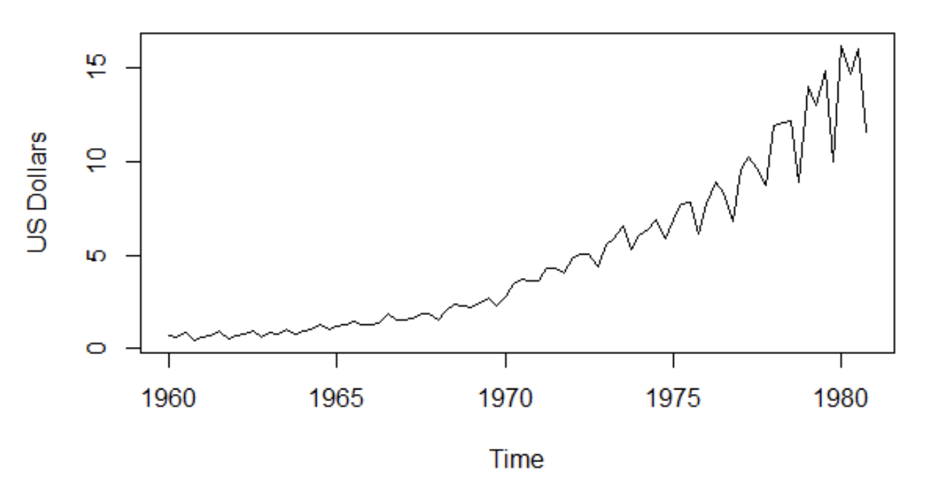
We clearly see that the series follows an increasing trend and a seasonal component.
Stationary Processes
Stationary processes are series which some of their properties do not vary with time.
Linear processes
All stationary processes can be represented a follow
$$ X_t = \mu + \sum^{\infty}_{i = -\infty} \psi_i W_{t - i} $$
for all $t$.
$\mu \in \mathbb{R}$, $\left\{ \psi_i \right\}$ is an absolutely summable sequence of constants and $\left\{ W_i \right\}$ is a white noise series with mean $0$ and variance $\sigma^2$.
Absolutely summable sequence
For a sequence to be absolutely summable, the following condition needs to be met:
$$ \sum^{\infty}_{n = -\infty} |a_n| \lt \infty $$
We define the backward shift operator, $B$, as
$$ BX_t = X_{t - 1} $$
and
$$ B^iX_t = X_{t - i} $$
Linear processes can also be represented as
$$ X_t = \mu + \psi(B) W_t $$
where
$$ \psi(B) = \sum^{\infty}_{i = -\infty} \psi_i B^i $$
The mean of the linear process is $\mu$ and its covariance function is given by:
$$ \gamma(h) = \text{Cov}(X_t, X_{t+h}) = \text{Cov}(\mu + \sum^{\infty}_{i = -\infty} \psi_i W_{t - i}, \mu + \sum^{\infty}_{i = -\infty} \psi_i W_{t + h - i}) $$
$$ \gamma(h) = \sum^{\infty}_{i = -\infty} \psi_i \psi_{i + h} \text{Cov}(W_{t - i}, W_{t - i}) = \sigma^2 \sum^{\infty}_{i = -\infty} \psi_i \psi_{i + h} $$
since $\text{Cov}(W_{t - i}, W_{t + h - i}) = 0$ if $t - i \neq t + h - i$.
A linear process is said to be causal or a causal function of $\left{ Z_t \right}$ if there exists constants $\left{ \psi_i \right}$ such that $\sum^{\infty}_{i = 0} |\psi_i| \lt \infty$ and:
$$ X_t = \sum^{\infty}_{i = 0} \psi_i W_{t - i} $$
for all $t$.
A linear process is invertible if there exists constants $\left\{ \pi_i \right\}$ such that $\sum^{\infty}_{i = 0} |\pi_i| \lt \infty$ and:
$$ W_t = \sum^{\infty}_{i = 0} \pi_i X_{t - i} $$
for all $t$.
AR process
Autoregressive models are based on the idea that the current value can be expressed as a combination of previous values of the series plus a random component.
Let $\left\{ X_t \right\}$ be a time series and $\left\{ W_t \right\}$ a white noise series. An autoregressive model of order p is defined as:
$$ X_t = c + \sum_{i = 1}^{p} \phi_i X_{t - i} + W_t $$
Where $\phi_i$ are constants and $\phi_p \neq 0$.
Using the backward shift operator, we can rewrite the previous expression as:
$$ X_t = c + \phi_1 B X_{t - 1}+ \phi_2 B^2 X_{t-2} + … + \phi_p B^p X_{t - p} + W_t $$
Sometime the following concise notation is used:
$$ \phi(B)X_t = W_t $$
where $\phi(B) = 1 - \phi_1 B - \phi_2 B^2 - … - \phi_p B^p$.
The $\text{AR}(1)$ process is then given by:
$$ X_t = c + \phi X_{t - 1} + W_t $$
Stationarity of the $\text{AR}(1)$ process
Let’s first compute the mean of $\text{AR}(1)$:
$$ \mu(X_t) = \mu(c + \phi X_{t - 1} + W_t) $$
$$ \mu(X_t) = \mu(c) + \mu(\phi X_{t - 1}) + \mu(W_t) $$
$$ \mu(X_t) = c + \phi \mu(X_{t - 1}) $$
For the process to be stationary, its mean needs to be unchanged over time, which means $\mu(X_t) = \mu(X_{t-1})$:
$$ \mu(X_t) = c + \phi \mu(X_t) $$
$$ \mu(X_t)(1 + \phi) = c $$
$$ \mu(X_t) = \frac{c}{1 - \phi} $$
Which means that $\mu(X_t) < \infty$ as long as $\phi \neq 1$.
Also, it gives us a condition for the process to be stationary, linking both $\phi, c$.
Let’s look at its variance:
$$ \text{Var}(X_t) = \text{Var}(c + \phi X_{t - 1} + W_t) $$
$$ \text{Var}(X_t) = \phi^2 \text{Var}(X_{t - 1}) + \text{Var}(W_t) + 2\text{Cov}(\phi X_{t - 1}, W_t) $$
$X_{t - 1}, W_t$ are independent so:
$$ \text{Var}(X_t) = \phi^2 \text{Var}(X_{t - 1}) + \sigma^2 $$
For the process to be stationary, its variance needs to stay the same over time:
$$ \text{Var}(X_t) = \phi^2 \text{Var}(X_{t}) + \sigma^2 $$
We get the following condition for the variance:
$$ \text{Var}(X_t) = \frac{\sigma^2}{1 - \phi^2} $$
Remember that we also know that: $c = (1 - \phi)\mu(X_t)$, we can then center the process:
$$ X_t - \mu(X_t) = \phi(X_{t - 1} - \mu(X_t)) + W_t $$
We will use this result to compute the autocovariance function.
$$ \gamma(h) = \text{Cov}(X_t, X_{t - h}) $$
Note that we used $t - h$ instead of $t + h$ which makes no difference because we can just use $t \leftarrow t + h$ and swap $X_t$ with $X_{t + h}$.
$$ \gamma(h) = E[(X_t - \mu)(X_{t - h} - \mu)] $$
$$ \gamma(h) = E[(\phi(X_{t - 1} - \mu) + W_t)(X_{t - h} - \mu)] $$
$$ \gamma(h) = E[(\phi (X_{t - 1} - \mu))(X_{t - h} - \mu)] + \text{Cov}(W_t, X_{t - h}) $$
$$ \gamma(h) = \phi \text{Cov}(X_{t - 1}, X_{t - h}) $$
$$ \gamma(h) = \phi \gamma(h - 1) $$
By iterating:
$$ \gamma(h) = \phi^h \gamma(0) = \phi^h \text{Var}(X_t) $$
We already computed the value of the variance:
$$ \gamma(h) = \phi^h \frac{\sigma^2}{1 - \phi^2} $$
Based on the values of the mean, the variance and the autocorrelation, we can say that the process is weakly stationary if:
$$ |\phi| < 1 $$
MA process
The idea behind moving average processes is that current values can be expressed as a linear combination of the current white noise and the $q$ most recent past white noise terms.
Let $\left\{ X_t \right\}$ be a time series and $\left\{ W_t \right\}$ be a white noise series. A moving average model of order q is defined as:
$$ X_t = W_t - \theta_1 W_{t - 1} - … - \theta_q W_{t - q} $$
Using the backshift operator:
$$ X_t = \theta(B)W_t $$
Where $\theta(B) = 1 - \theta_1 B - … - \theta_q B^q$.
The $\text{MA}(1)$ process is then given by:
$$ X_t = W_t - \theta W_{t - 1} $$
The condition for stationarity is always fulfilled:
- $\mu(X_t) = 0$
- $\gamma(0) = \text{Var}(X_t) = \sigma^2(1 - \theta^2)$
- $\gamma(1) = \text{Cov}(X_t, X_{t - 1}) = -\theta \sigma^2$
- $\gamma(h) = \text{Cov}(X_t, X_{t - h}) = E[(W_t - \theta W_{t - 1})(W_{t - h} - \theta W_{t - h - 1})] = 0$ if $h > 1$
ARMA process
Autoregressive models and moving average models take into account different kinds of dependencies between observations over time.
We can mix those two types of models into one.
Let $\left\{ X_t \right\}$ be a time series and $\left\{ W_t \right\}$ a white noise series. An autoregressive moving average process of order (p, q) is defined as:
$$ X_t = \phi_1 X_{t - 1} + … + \phi_p X_{t - p} + W_t - \theta_1 W_{t - 1} - … - \theta_q W_{t - q} $$
It can be written as:
$$ (1 - \sum_{i=1}^{p} \phi_i B^i) X_t = (1 - \sum_{i=1}^{q} \theta_i B^i)W_t $$
Using the backward shift operator, the process can be expressed as:
$$ \phi(B)X_t = \theta(B)W_t $$
Where: $\phi(B) = 1 - \phi_1 B -…- \phi_p B^p$ and $\theta(B) = 1 - \theta_1 B - … - \theta_p B^p$.
The $\text{ARMA(1, 1)}$ process is given by:
$$ X_t = \phi X_{t - 1} + W_t - \theta W_{t - 1} $$
- Its stationary condition is $\phi \neq 1$
- Its causal condition is $|\phi| < 1$
- Its invertibility condition is $|\theta| < 1$
The autocovariance function is:
$$ \gamma(0) = \frac{\sigma^2(1 + \theta^2 - 2 \phi \theta)}{1 - \phi^2} $$
$$ \gamma(1) = \frac{\sigma^2(1 - \phi \theta)(\phi - \theta)}{1 - \phi^2} $$
$$ \gamma(h) = \phi \gamma(h - 1) = \phi^{h - 1}\gamma(1) $$
if $h > 1$.
Non-stationary Processes
Some time series are not stationary because of trends or seasonal effects.
A time seres that is non stationary because of a trend can be differentiated into a stationary time series. Once differentiated it is possible to fit an ARMA model on it.
This kind of processes is called autoregressive integrated moving average (ARIMA) since the differentiated series needs to be summed or integrated to recover the original series.
ARIMA was introduced in 1955.
The seasonal component of a time series is the change that is repeated cyclically over time and at the same frequency. The ARIMA model can be extended to take into account the seasonal component. This is done by adding additional parameters. In this case, it is known as seasonal autoregressive integrated moving average models (SARIMA).
ARIMA process
A time series that is not stationary in terms of mean can be differentiated as many times as needed until stationary. It is done by substracting the previous observation to the current observation, we are not talking about computing the derivative here.
We define the differential operator $\nabla$:
$$ \nabla := (1 - B) $$
And
$$ \nabla X_t = (1 - B)X_t = X_t - X_{t - 1} $$
Let’s take an example: the random walk. This process is defined as :
$$ X_t = X_{t - 1} + W_t $$
We saw that this process is not stationary, but we can differentiate it:
$$ \nabla X_t = X_{t - 1} + W_t - X_{t - 1} = W_t $$
which is stationary.
Let $\left\{ X_t \right\}$ be a time series and $d$ a positive integer. $\left\{ X_t \right\}$ is an autoregressive integrated moving average model of order (p, d, q) if:
$$ Y_t = (1 - B)^d X_t $$
is a causal $\text{ARMA(p, q)}$ process.
Substituting $Y_t$, we get:
$$ \phi(B)(1 - B)^d X_t = \theta(B) W_t $$
It basically means that an ARIMA(p, d, q) series is a series that after being differentiated d times, is an ARMA(p, q) series.
The p is the order of the autoregressive part, the q is the order of the moving average part and the d is the number of times we differentiate the series.
Note that if $d = 0$, this model represents a stationary ARMA(p, q) process.
We say that a series is integrated of order $d$ if it is not stationary but its $d$ difference is stationary. Fitting an ARMA model to an integrated process is known as fitting an ARIMA model.
Let’s give some examples.
ARIMA(1, 1, 0)
The ARIMA(1, 1, 0) is a simple ARIMA model where the process is made of a series that after being differentiated one time is a autoregressive model with no moving average part.
ARIMA(0, 1, 1)
The ARIMA(0, 1, 1) is a simple ARIMA model where the process is made of a series that after being differentiated one time is a moving average model with no autoregressive part.
SARIMA process
We give the SARIMA process definition for information purposes only, we won’t discuss it in details.
Let $\left\{ X_t \right\}$ be a time series and $d, D$ positive integers. $\left\{ X_t \right\}$ is a seasonal autoregressive integrated moving average model of order (p, d, q) with period s if the process $Y_t = (1 - B)^d(1 - B^2)^DX_t$ is a causal $\text{ARMA}$ process defined by:
$$ \phi(B)\Phi(B^s)Y_t = \theta(B)\Theta(B^s)W_t $$
with $\phi(B) = 1 - \phi_1 B -…- \phi_p B^p$, $\Phi(B^s) = 1 - \Phi B^s -…- \Phi B^{Ps}$, $\theta(B) = 1 - \theta_1 B - …- \theta_pB^p$, $\Theta(B^s) = 1 - \Theta_1 B - …- \Theta_Q B^{Qs}$.
Model Selection
The main reason of modeling time series is for forecasting purposes. Therefore it is necessary to know which model is best for a specific time series.
The procedure of identifying a worthy model for our time series follows these steps:
- Identify a model
- Estimate the parameters of the model
- Check if the model fits well the data
- If yes, we keep the model, if not we go back to step 1
Model identification
Here we are trying to find a model that could potentially fit our data. The first thing to do is fit an ARMA model to make sure that our data is stationary in mean.
If the data are not stationary in mean, we differentiate it until it is. If the data is not stationary in variance, then a specific transformation can be applied: the Box and Cox power transformation.
Let $\left\{ X_t \right\}$ be a time series. We define the Box-Cox transformation $f_{\lambda}$ as:
$$ f_{\lambda}(X_t) = \begin{cases} \frac{X_t^{\lambda} - 1}{\lambda} & \text{ if } \lambda > 0 \ \ln X_t & \text{ if } \lambda = 0 \end{cases} $$
Where $\lambda$ is a real parameter.
Most of the time, we use $\lambda = 0$.
The transformation has to be applied before differentiation.
Parameters estimation
Once a feasible model has been identified we have to estimate its parameters.
One of the most used method for parameters estimation is the well known maximum likelihood estimation method. This method estimates the parameters that maximise the probability of the observed data. The parameters are the ones with the highest probability of generating the data.
Let $\left\{ X_t \right\}$ be a time series and $\Gamma_n$ the covariance matrix. Assuming that $\Gamma_n$ is non singular, the function of likelihood of $X_t$ is:
$$ L(\Gamma_n) = (2\pi)^{-n/2} \text{det}(\Gamma_n)^{-1/2} \exp(-\frac{1}{2}X_n\Gamma_n^{-1}X’_n) $$
Note that the covariance matrix depends on the values of the parameters, so it depends on the chosen model.
In case $\left\{ X_t \right\}$ is univariate, the function of likelihood becomes:
$$ L(X_t) = \frac{1}{(2\pi)^{n/2} \sigma^n}\exp(- \frac{1}{2 \sigma^2} \sum (X_i - \mu)^2) $$
Practically, we will assume the noise $\left\{ W_t \right\}$ follows a normal distribution $N(0, \sigma^2)$. This is why we can get such a likelihood function.
Once we have this likelihood function, we will take its logarithm. Because the logarithm is a monotonic function, it does not change the value of the minimum.
Then, we compute the derivative of the logarithm of the likelihood with respect to the variance of the white noise. Finally, we search for the values of the parameters that minimise this derivative.
Resolution for AR(1)
Let us take $X_t = \phi X_{t - 1} + W_t$ with $W_t \sim N(0, \sigma^2)$.
One can write that:
$$ X_t|X_{t - 1} \sim N(\phi X_{t-1}, \sigma^2) $$
And then give the conditional likelihood:
$$ L(X|X_{-1}) = \prod^{T}{i = 2}L(x_i|x{i - 1}) $$
$$ L(X|X_{-1}) = (\sigma^2 2 \pi)^{-\frac{T - 1}{2}}\exp(-\frac{1}{2 \sigma^2} \sum^T_{i = 2}(x_i - \phi x_{i - 1})^2) $$
Then after applying the log on it:
$$ \log L(X|X_{-1}) = -\frac{T - 1}{2} (\log 2 \pi + \log \sigma^2) - \frac{1}{2 \sigma^2}\sum^T_{i = 2}(x_i - \phi x_{i - 1})^2 $$
Once we have the log likelihood expression, we need to compute its derivative with respect to $\sigma$ and find the best values for the parameters $\sigma, \phi$.
Here is an interesting paper about the resolution for ARMA(1, 1):
Model diagnostic
Finally, once we have a model and its corresponding parameters, we need to make sure that the model is adequate.
In order to find the model with the highest potential of “good fitting”, we can use the Akaike Information Criterion. This criterion evaluates the quality of the model relatively to other models based on the information that is lost by using the model instead of others.
Let $\left\{ X_t \right\}$ be a time series and $L$ be the likelihood function of the model. The Akaike information criterion is given by:
$$ AIC = 2k - 2\ln(L) $$
With k the number of parameters in the model.
The model that minimises the loss information is the minimum $AIC$ model.
Conclusion
Even though the previous methods are relatively simple, they tend to work very well on time series. Learning them provides us with benchmarks to compare the performance of our deep learning models.
Because most of the time deep learning relies on very big sets of parameters, we need to make sure that it offers a advantage over smaller models.
As a conclusion, here is a funny blog post about an extremely simple method to forecast financial time series.
The probable speculative constant
Additional Resources
General statistics & probability theory
Statlect, the digital textbook | Probability, statistics, matrix algebra
Probability Theory and Stochastic Processes
Parameters estimation
Miscellaneous
Practical Work
In order to put into practice what we just learnt, we are going to forecast the monthly number of air passengers.
Setup the notebook
Create a notebook and download the data that is located inside the Google Drive folder that you should have access to.
https://drive.google.com/file/d/154k9rmqAeg2JdOUyeE4kQKyykoAxivwZ/view?usp=sharing
You will need several libraries. Some of them come with python, some of them need to be installed manually.
import os
import numpy
import pandas
from scipy.stats import boxcox
from matplotlib import pyplot as plt
from statsmodels.tsa.arima.model import ARIMA
Read the data
In the same folder, you will also find the data file named data.csv.
It contains the monthly number of air passenger from 1949 to 1960.
The file itself is very simple, it contains only two columns, one with being the date and the second being the number of passengers.
Plot the data
Using matplotlib, plot the data inside the notebook. This should show a clear trend and seasonality.
Make the series stationary
To make sure the process is stationary, we need both to remove the seasonality and the trend. We will start by removing the seasonality using the Box-Cox transformation.
The transformation is available inside the scipy Python package.
from scipy.stats import boxcox
scipy.stats.boxcox — SciPy v1.11.3 Manual
Once the seasonality is remove, we can differentiate. Feel free to differentiate many times in order to see how this affects the data and at what point it seems stationary in mean.
You can differentiate manually using the .diff method of the pandas.DataFrame object (it is also available to the pandas.Series object).
pandas.DataFrame.diff — pandas 2.1.2 documentation
The .diff method is also available on numpy.array object.
numpy.diff — NumPy v1.26 Manual
Choose a model & estimate its parameters
Once the data is stationary, we need to choose a model and estimate its parameters.
This can be done using the statsmodels library that contains specific functions to work with ARIMA and ARMA models. Here is how you can import them:
from statsmodels.tsa.arima.model import ARIMA
You can notice that there is no ARMA specific import. It is so because the ARMA(p, q) model is equivalent to an ARIMA(p, 0, q) model.
And the documentation:
statsmodels.tsa.arima.model.ARIMA - statsmodels 0.14.0
Fitting a model using this library will return an object that you can use to display a summary:
print(result.summary())
Inside the summary, you will find the value of the AIC criterion.
You have to try many values for p and q (if you are sure that d is the right one after differentiation) and choose the best values for both of them based on the value of the AIC criterion.
Analyse the results
Finally, in order to evaluate the results, you can forecast using the model you just fit. A method get_forecast exists for the result of the fit method of the ARIMA object.
You can use it to get the next values of the time series.
Once you managed to forecast, you can get to the original data back by retransforming the data to the original non-stationary series.
The differentiation depends on the value of the d parameters your fitting gave.
The Box-Cox transformation can be reverted using the scipy library again:
from scipy.special import inv_boxcox