Differentiable Clustering
Problem Formulation
Let $\mathcal{X} = \{x_1, x_2, \dots, x_N\}$ denote a dataset of $N$ items, where each $x_i \in \mathbb{R}^d$ is a dense embedding vector representing a text tag. Our objective is to partition $\mathcal{X}$ into $k$ distinct clusters.
We define a differentiable, parametric mapping
$$ f_\theta : \mathbb{R}^d \rightarrow \Delta^{k-1} $$where $\Delta^{k-1}$ is the standard $(k - 1)$-dimensional probability simplex. The function $f_\theta$ is defined as a linear projection followed by a softmax activation:
$$ p_i = f_\theta(x_i) = \text{softmax}(W x_i + b) $$Where:
- $W \in \mathbb{R}^{k \times d}$ and $b \in \mathbb{R}^k$ are the learnable parameters $\theta = \{W, b\}$
- The output $p_i \in [0,1]^k$ represents the probability distribution of item $i$ over the $k$ clusters, such that $\sum_{c=1}^k p_{i,c} = 1$
Unsupervised Structural Alignment
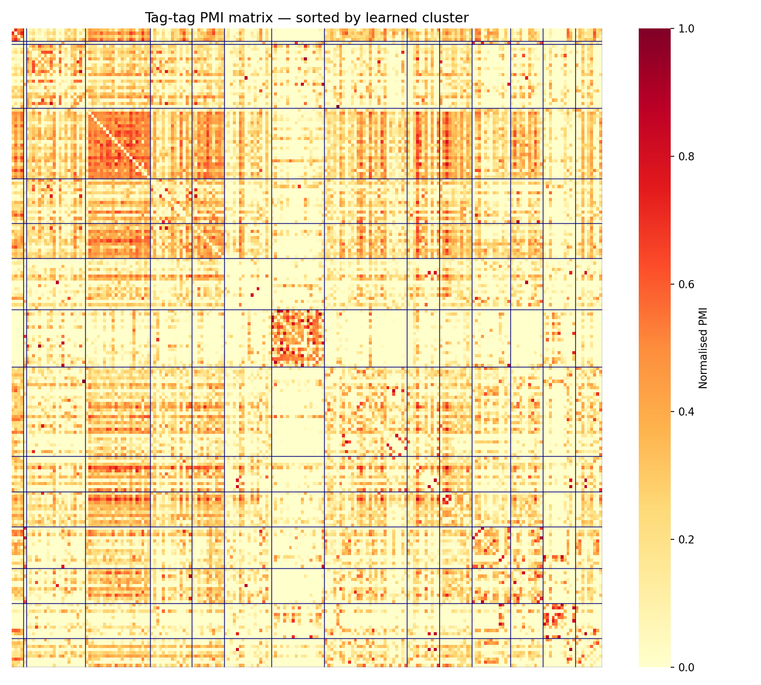
We already know that some tags are closer than others. The mutual information metric tells us that some tags appear often together, and so we might want to keep them closer. We utilize a pre-computed pairwise mutual information matrix $M \in \mathbb{R}^{N \times N}$. The element $M_{ij}$ quantifies the co-occurrence between $x_i$ and $x_j$.
We optimize the network such that the inner product of the soft assignments $p_i^\top p_j$ is maximized when $M_{ij}$ is high. For a given mini-batch $\mathcal{B}$, the structural alignment loss is formulated as:
$$ \mathcal{L}_{align} = - \frac{1}{|\mathcal{B}|^2} \sum_{i,j \in \mathcal{B}} M_{ij} (p_i^\top p_j) $$The PMI matrix below is computed on the top-200 tags from the Last.fm HetRec dataset, ordered by learned cluster. The block-diagonal structure shows that the model successfully groups co-occurring tags (metal subgenres, rock variants, electronic/ambient tags, and pop genres) each forming tight blocks.
Entropy Regularization
To prevent trivial mode collapse (where the network collapses all embeddings into a single cluster to superficially minimize $\mathcal{L}_{align}$), we introduce an entropy regularization term.
Let $\bar{p} = \frac{1}{|\mathcal{B}|} \sum_{i \in \mathcal{B}} p_i$ be the marginal cluster assignment distribution over the mini-batch. We penalize low entropy in this marginal distribution to ensure all $k$ clusters are utilized approximately equally:
$$ \mathcal{L}_{entropy} = \sum_{c=1}^k \bar{p}_c \log(\bar{p}_c) $$Minimizing this term (which is equivalent to maximizing the Shannon entropy of $\bar{p}$) encourages a uniform prior over the cluster sizes.
Semi-Supervised Constraints
We have a tool to manually review clusters. For each cluster, we can decide whether it is coherent or not, and if it isn’t, we can tag it as:
- Too narrow: should be merged into another cluster
- Too broad: should be split
- Geo-specific: should be merged into another cluster as well
When marking a cluster as too broad, we are giving explicit ordering signals to the optimization process. To inject this into the optimization procedure, we define two additional constraint sets:
- Must-Link Set $\mathcal{S}$: A set of pairs $(i, j)$ that must belong to the same cluster.
- Cannot-Link Set $\mathcal{D}$: A set of pairs $(i, j)$ that must be assigned to disjoint clusters.
We penalize deviations from these constraints using the following loss terms:
$$ \mathcal{L}_{ML} = \frac{1}{|\mathcal{S}|} \sum_{(i,j) \in \mathcal{S}} \|p_i - p_j\|_2^2 $$$$ \mathcal{L}_{CL} = \frac{1}{|\mathcal{D}|} \sum_{(i,j) \in \mathcal{D}} (p_i^\top p_j) $$The must-link loss $\mathcal{L}_{ML}$ minimizes the Euclidean distance between probability distributions of anchored pairs, while the cannot-link loss $\mathcal{L}_{CL}$ forces their assignment vectors to be orthogonal.
Geometric Smoothness Regularization
While the structural alignment loss $\mathcal{L}_{align}$ captures discrete topological relationships (e.g., co-occurrence or mutual information), it does not explicitly account for the continuous spatial relationships within the embedding space $\mathcal{X}$.
To enforce local consistency (ensuring that vectors strictly proximate in the embedding space are assigned to the same cluster), we introduce a geometric smoothness penalty based on graph Laplacian regularization.
First, we define a continuous similarity matrix $S \in \mathbb{R}^{N \times N}$ over the embedding space. A standard choice is the Gaussian Radial Basis Function (RBF) kernel applied to the Euclidean distance between embeddings:
$$ S_{ij} = \exp\left(-\frac{\|x_i - x_j\|_2^2}{2\sigma^2}\right) $$Where $\sigma$ is a scaling parameter (bandwidth) that controls the radius of the local neighborhood. If $x_i, x_j$ are very close, $S_{ij} \approx 1$. As the distance increases, $S_{ij} \rightarrow 0$.
We then formulate a loss term that penalizes diverging probability assignments for geometrically similar vectors. For a mini-batch $\mathcal{B}$, the geometric smoothness loss is defined as:
$$ \mathcal{L}_{geom} = \frac{1}{|\mathcal{B}|^2} \sum_{i,j \in \mathcal{B}} S_{ij} \|p_i - p_j\|_2^2 $$Minimizing $\mathcal{L}_{geom}$ forces the soft assignment vectors $p_i, p_j$ to converge when their source embeddings $x_i, x_j$ are close in the manifold. Alternatively, this can be formulated using the inner product to match $\mathcal{L}_{align}$:
$$ \mathcal{L}_{geom} = - \sum_{i,j \in \mathcal{B}} S_{ij}(p_i^\top p_j) $$yielding a similar optimization landscape.
Final Objective Function
Integrating the geometric constraint into our previous formulation yields a robust objective that simultaneously optimizes for global co-occurrence, local spatial geometry, uniform cluster distribution, and semi-supervised human constraints:
$$ \mathcal{L}_{total}(\theta) = \mathcal{L}_{align} + \lambda_G \mathcal{L}_{geom} + \lambda_H \mathcal{L}_{entropy} + \lambda_{ML} \mathcal{L}_{ML} + \lambda_{CL} \mathcal{L}_{CL} $$Where $\lambda_G \in \mathbb{R}^+$ controls the strength of the manifold regularization.
Each component in this objective plays a distinct role:
- $M_{ij}$ (Mutual Information) captures semantic relationships: tags like “jazz” and “saxophone” may be far apart in embedding space but frequently co-occur, so the alignment loss pulls their cluster assignments together.
- $S_{ij}$ (Geometric Similarity) captures syntactic/vector proximity: tags like “jazz club” and “jazz clubs” are nearly identical in the embedding space and should trivially end up in the same cluster.
- $\mathcal{L}_{entropy}$ prevents degenerate solutions where all items collapse into a single cluster.
- $\mathcal{L}_{ML}$ and $\mathcal{L}_{CL}$ inject domain knowledge from human review directly into the optimization loop.
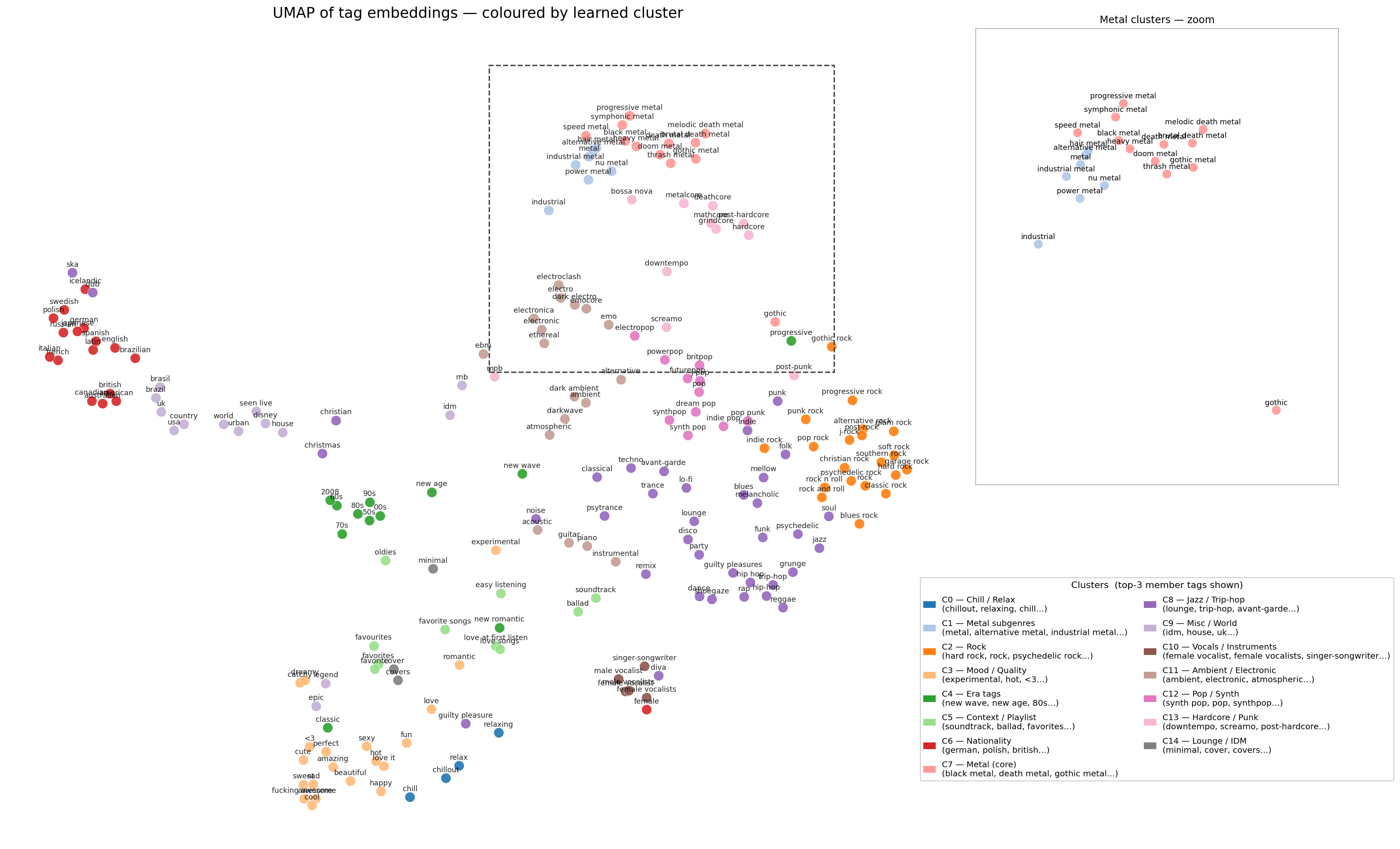
The UMAP below shows the result on the Last.fm tag dataset ($N=200$, $k=15$). Tags are embedded with all-MiniLM-L6-v2 and the model is warm-started with K-means centroids. The zoomed panel highlights how tightly the metal subgenres cluster together (progressive metal, symphonic metal, black metal, and doom metal all land in the same region despite having very different surface forms).
Search
Once the clusters are ready, they can be used for various downstream tasks. One of the most important is search: surfacing the most relevant activities from the catalog in response to a user query. Like clustering, search can be framed as a fully differentiable learning process.
Selecting the Right Cluster
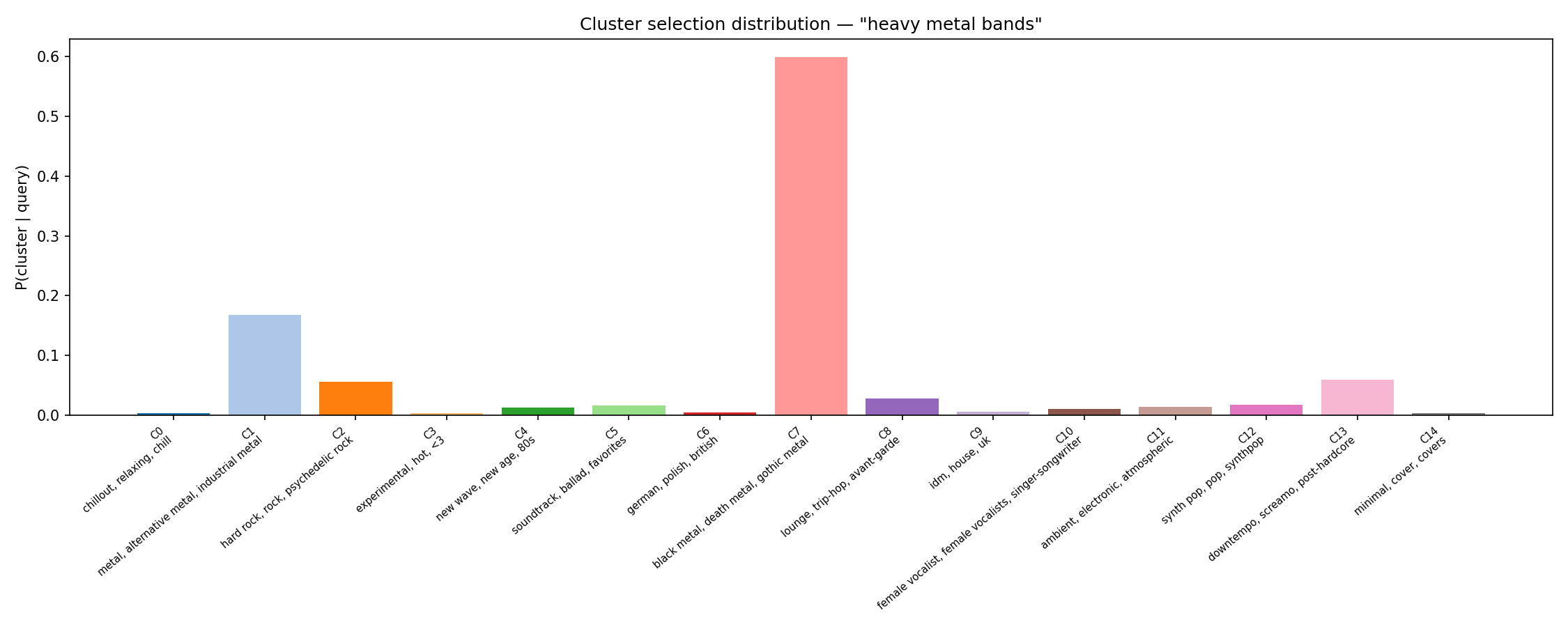
Rather than computing the distance to every cluster centroid and taking the closest one (which involves a non-differentiable $\argmax$), we define a probability distribution over all clusters given a query $q$:
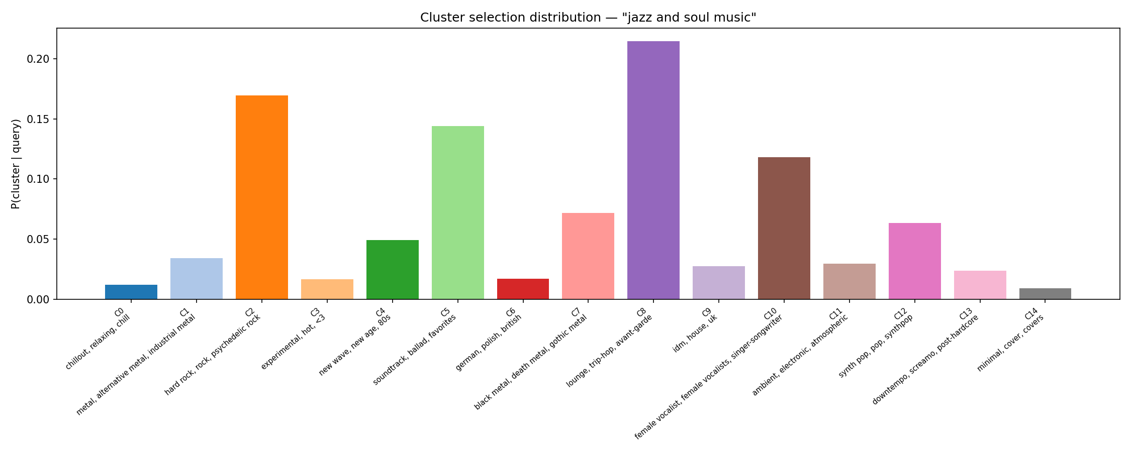
$$ P(c_j | q) = \frac{\exp(E(q) \cdot c_j / \tau)}{\sum_{i=1}^k \exp(E(q) \cdot c_i / \tau)} $$Here $E(q)$ is the embedding of the query, $c_j$ is the representation of cluster $j$, and $\tau$ is a temperature parameter controlling the sharpness of the distribution. As $\tau \rightarrow 0$ this recovers the hard nearest-cluster assignment; as $\tau$ grows the distribution becomes uniform.
The probability of a specific activity $a$ being relevant to query $q$ is then:
$$ P(a|q) = \sum_{j=1}^k P(c_j | q) \, W_{a \cdot c_j} $$where $W_{a \cdot c_j}$ is a scoring function encoding the association between activity $a$ and cluster $c_j$. This formulation is fully differentiable end-to-end.
The two figures below show the cluster selection distribution $P(c|q)$ for two example queries. The model correctly concentrates probability mass on the metal cluster for a metal query, and on the jazz/trip-hop cluster for a jazz query.
Ground-Truth Data and Loss Function
To train this system, we need an objective. We frame our labeled dataset as:
$$ \mathcal{D} = \left\{ (q_1, a_1^+),\ (q_2, a_2^+),\ \ldots \right\} $$where each pair $(q_i, a_i^+)$ consists of a user query and an activity that should rank highly for that query. For each query $q_i$, we want $P(a_i^+ | q_i)$ to be as high as possible and the probability of irrelevant activities $P(a_i^- | q_i)$ to be as low as possible.
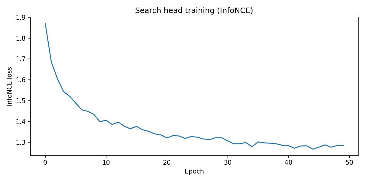
We use the InfoNCE loss:
$$ \mathcal{L} = -\log \frac{\exp(S(q, a^+))}{\exp(S(q, a^+)) + \sum_{a^-} \exp(S(q, a^-))} $$where $S(q, a)$ is the relevance score of activity $a$ for query $q$ as computed by the model above. This is the standard contrastive loss used in dense retrieval: the model is trained to score the positive activity higher than all negatives in the batch.
The choice of negatives matters significantly in practice. Random in-batch negatives are easy to distinguish; hard negatives (activities that are plausible but wrong) are what push the model toward precise retrieval.
The training curve below shows the InfoNCE loss on the Last.fm dataset, using tag names as pseudo-queries and the artists most associated with each tag as positives.