When fine tuning or even training a model, hardware resources are often the bottleneck, and with today’s model sizes, the limiting factor is often GPU memory.
As an example, let’s take a Qwen 2.5 3B models. As the name says, it contains approximately 3 billion parameters. The model available on HuggingFace is saved with bf16, meaning it contains:
- Sign bit : 1 bit
- Exponent : 8 bits
- Significant precision : 7 bits
So the total size in memory for 1 parameter among the 3 billion is 16 bits, which is 2 bytes. To store the whole model, the memory will need to be at least 6 billion bytes (6Gb).
But of course we cannot just store the model, we have to store the training data as well, the intermediary results of the computation throughout the neural network, and even the gradients in order to be able to train the model.
As an example, let’s take a toy neural network that contains 2 layers. The model would look like that:
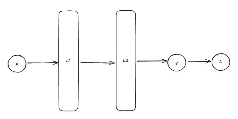
Where:
- $x \in X$ is the input data
- $L_1, L_2$ are the two layers, containing parameters $\theta_1, \theta_2$ respectively
- $y$ is the output of the neural network
- $L$ is the value of the loss function
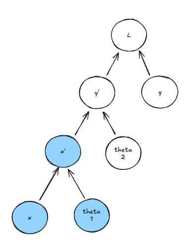
Every time we want to compute $\hat{y}$ from $x$ we have to go through this computation graph:

Where :
- $\theta_1 \in \mathbb{R}^{d \times d_1}$ the parameters of the first layer
- $\theta_2 \in \mathbb{R}^{d_1 \times d_2}$ the parameters of the second layer
- $x \in \mathbb{R}^{b \times d}$ is the input data as in the previous figure
- $b$ is the batch size
- $d$ is the dimension of the data
- $x’ \in \mathbb{R}^{b \times d_1}$ is the intermediary result $x’ = f^1_{\theta_1}(x)$
- $\hat{y} \in \mathbb{R}^{b \times d_2}$ is the prediction (written $y’$ in the figure) given by $\hat{y} = f^2_{\theta_2}(x’)$
- $y \in \mathbb{R}^{b \times d_2}$ is the ground truth
- $L = L(\hat{y}, y) \in \mathbb{R}$ is the loss
The graph indicates what input nodes are required to compute any node. So for example, to compute the prediction, we have to have the intermediary result and the parameters of the second layer loaded in memory.
If we want to load the whole graph into memory to perform a forward pass, we then have to load all the previous tensors, which means storing in memory:
- $d * d_1 * 2$ bytes for $\theta_1$
- $d_1 * d_2 * 2$ bytes for $\theta_2$
- $b * d * 2$ bytes for $x$
- $b * d_1 * 2$ bytes for $x'$
- $b * d_2 * 2$ bytes for $\hat{y}$
- $b * 2$ bytes for $L$
Considering the following values:
| b | 32 |
|---|---|
| d | 1000 |
| d1 | 1000 |
| d2 | 1000 |
Gives 4.192.032 bytes. Among that, the two layers of the models (the parameters) account for 4.000.000 bytes.
Now that we understand the context a bit more clearly, let’s talk about how we can reduce the memory footprint.
Gradient Accumulation
As we saw in the toy example, we are working with batches of data. Instead of sampling one example, running it through the network, computing the loss, the gradients and updating the model, we do it for a few examples at a time. It improves convergence and stabilize training.
But it comes with a cost, which is more memory required to work. Instead of loading 1 example of size 1000 (in the previous case), we have to load 32 examples of size 1000.
And things get worse if we are talking about a language model. A language model works with a few tokens, let’s say 1024, and each token is then embedded in a tensor of size depending on the model provider. For example, DeepSeek-v3 and R1 use an embedding of size 7168. So when we batch the data, we actually create tensors of size $b * 1024 * 7168 = 7 340 032 * b$. Which is a lot!
In this case, using a small batch or a big batch can make a huge difference in terms of memory usage.
This is where gradient accumulation comes into play.
Instead of loading the whole batch into memory, gradient accumulation loads only a fraction of a batch (for example 4 training samples instead of 32), performs the forward pass and compute the gradient of the loss function. It then loads another fraction of the batch, does the same operation on it and “accumulates” the gradient until a certain point is reached.
Then, after the accumulation steps, the optimizer can update the weights as if the gradients had been computed on the whole batch.
The whole point here is that we do not have to load the whole batch at once. So instead of loading $7 340 032 * 32 = 234.881.024 = 234 \text{Mb}$ we can only load one eighth of that.
Gradient Checkpointing
Gradient checkpointing is a bit trickier to understand.
Pebbles
To understand memory requirements of computation, computer scientists use the concept of pebble game, introduced in 1975 in a paper called “Complete Register Allocation Problems” !
In order to compute each value inside a computation graph (like the one we showed previously), we need to first load its dependencies in memory. The pebble game represents this as placing a pebble on the dependency nodes of the value we want to compute. If all dependency nodes have pebbles on them, all the required values are stored in memory and the node is ready for execution. Of course, when computing the node, we store its value into memory, so we place a pebble on it as well.
And like memory, we have a finite set of pebbles ! Meaning that we need to be smart when placing the pebbles, and making sure we are not leaving a pebble on a node that is not needed anymore.
Let’s recall the computation graph we used earlier. If we want to compute the $x’$ node, we would have to load the value $x$ and the parameters $\theta_1$ in memory which are its dependencies:
Once the two children values loaded, we can compute $x’$. Now moving forward to the second node to be computed : $\hat{y}$. We again need to load its children, but $x’$ is already loaded, so $\theta_2$ needs a pebble:
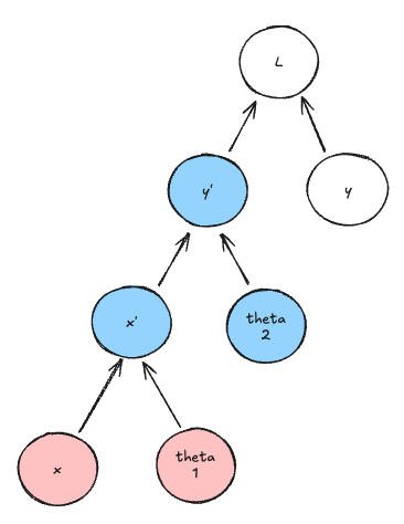
It is easy to notice that the two children nodes that we loaded into memory earlier are not needed anymore. So $x$ and $\theta_1$ can be freed, and their pebbles can be reclaimed.
And we will go all the way up to the loss function. Because no node has more than 2 dependencies, we can reach the loss function with only 3 pebbles instead of 7 if we keep the whole graph stored in memory.
Checkpointing
Now that we understand clearly how we can optimize memory consumption by freeing the nodes that are not directly needed for computation, we can get back to our original problem.
We know what it is possible to store only the immediate children nodes for the forward pass. But when training or fine tuning a model, we need to be able to compute the gradients and retropropagate them through the network.
The same logic can be applied to the backward pass. Indeed, to compute the gradient of the loss function with respect to node $x’$ for instance, we have to compute the gradient of the loss wrt $\hat{y}$ first, then use it as a child node.
To update the weights of the model, we need to compute two gradients :
- $\frac{\partial L(\hat{y}, y)}{\partial \theta_2}$
- $\frac{\partial L(\hat{y}, y)}{\partial \theta_1}$
The first expression is easy to compute :
$$ \frac{\partial L(\hat{y}, y)}{\partial \theta_2} = \frac{\partial L(\hat{y}, y)}{\partial \hat{y}} \frac{\partial \hat{y}}{\partial \theta_2} $$
We notice the gradient of the loss with respect to the prediction $\hat{y}$.
Then the second formula :
$$ \frac{\partial L(\hat{y}, y)}{\partial \theta_1} = \frac{\partial L(\hat{y}, y)}{\partial \hat{y}} \frac{\partial \hat{y}}{\partial x’} \frac{\partial x’}{\partial \theta_1} $$
This one is interesting because we see 3 gradients :
- the gradient of the loss wrt the prediction
- the gradient of the prediction wrt the intermediary $x'$
- the gradient of the intermediary node wrt the parameters of the first layer
To calculate this, you need the value of the intermediate activation $x’$, which was computed during the forward pass. The standard approach is to store all these activations in memory during the forward pass so they are available for the backward pass. For very deep models with many layers, these stored activations can consume an enormous amount of memory — often more than the model weights themselves.
The solution : Re-compute, don’t store
Gradient checkpointing takes a radical approach: it avoids storing most of the intermediate activations during the forward pass.
- Forward Pass: As the model executes the forward pass, it calculates all the activations but immediately discards most of them to free up memory. It only saves a few strategically chosen activations, called “checkpoints”. The kept nodes can be decided by the framework or even manually. Usually, around $\sqrt{n}$ nodes are kept.
- Backward Pass: When the backward pass needs an intermediate activation that was discarded, the model doesn’t have it. Instead, it recomputes it on the fly. It takes the most recently saved checkpoint and runs a partial forward pass from that checkpoint up to the point where the required activation is produced.
By re-running small segments of the forward pass during the backward pass, the model can avoid storing the bulk of the activations. This dramatically reduces memory usage at the cost of some re-computation, making it possible to train much larger models on the same hardware.